

Executive Summary
LogiAI turned a feasible routing plan into a lower-burden dispatch decision.
A last-mile delivery team needed to route 76 time-windowed stops across the Greater Toronto Area. The baseline used a legacy west-side distribution depot, 13 vehicles, 24-unit capacity per vehicle, a 900-minute route-duration limit, and the balanced routing objective.
The baseline met every delivery window, but it was not an efficient operating answer. LogiAI produced a feasible plan with 100% on-time service, yet the plan required 13 routes, 762.7 km of travel, and 87.8 hours of aggregate route duration.
AI Explain reframed the result correctly: the weakness was not lateness, because time windows were hard constraints. The weakness was the cost of preserving that promise from the wrong dispatch footprint with tight vehicle capacity and geographically dispersed stops.
The team tested one controlled What-if branch: move dispatch to MIDTOWN_MICRO_HUB, raise vehicle capacity from 24 to 26, and consolidate the plan from 13 vehicles to 12 while preserving the same 76 stops, the same time windows, the balanced objective, and the 900-minute route-duration policy.
The variant improved the operating picture. Total distance dropped from 762.7 km to 598.7 km, total duration dropped from 87.8 h to 75.3 h, vehicles used dropped from 13 to 12, and on-time service stayed at 100%.
Distance
762.7 km to 598.7 km
Route duration
87.8 h to 75.3 h
Vehicles
13 to 12
Core capabilities exercised
- Single-depot CVRP optimization with stop demand, service duration, coordinates, and time-window inputs.
- Fleet controls for vehicle count, capacity per vehicle, route-duration limits, objective, runtime, and solver policy.
- Route map, KPI summary, route review, and route-level load/duration evidence for operational review.
- Hard time-window feasibility so the customer promise stays explicit during scenario comparison.
- AI Explain to interpret why a feasible routing plan is still operationally expensive.
- What-if Analysis to test depot and fleet-policy changes before saving a new scenario.
- AI Compare to evaluate deterministic KPI movement and summarize adoption trade-offs.
Operating context
The customer promise was protected, but the network design was expensive.
Vehicle routing is often judged incorrectly by one metric. If every delivery is on time, the route plan may look finished. In real operations, the same plan can still waste driver hours, mileage, fuel, and vehicle capacity.
This case represents a GTA delivery operation with customers spread across Downtown Toronto, North Toronto, East Toronto, West GTA, Markham, Oakville, and Brampton. Every stop has a numeric delivery window, demand quantity, service time, and coordinate location.
The operation started from a legacy west-depot footprint. That depot could support the plan, but it forced long cross-region route legs while the optimizer tried to keep every stop inside its hard appointment window.
LogiAI was used to separate feasibility from operating quality. The team needed to know whether the delivery promise could be preserved with a lower-distance and lower-duration plan before changing the dispatch strategy.
Challenge
The team needed lower route burden without relaxing time windows.
The baseline was intentionally feasible, not broken. That matters because many real routing decisions start after the team already has a plan that works on paper.
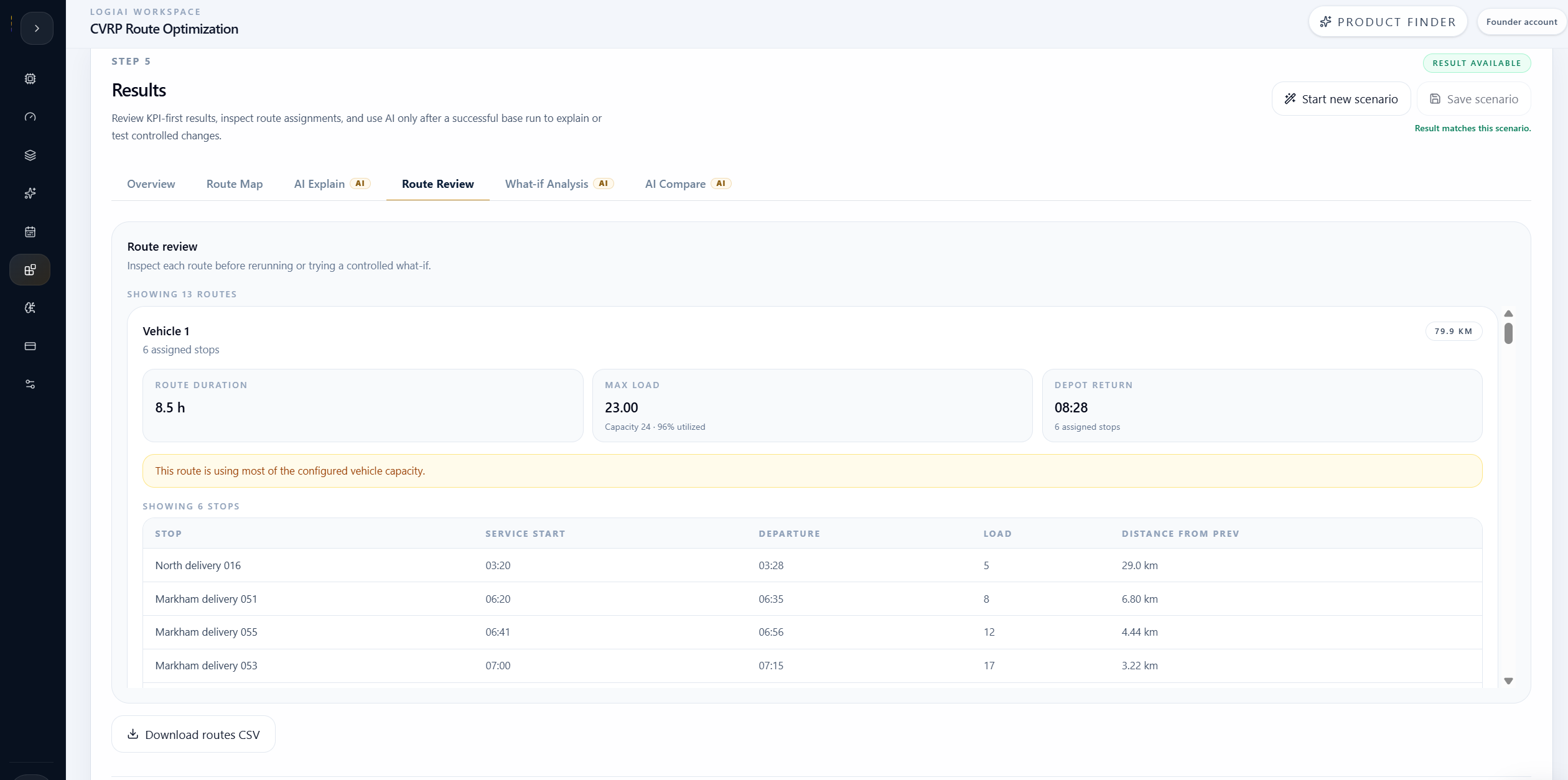
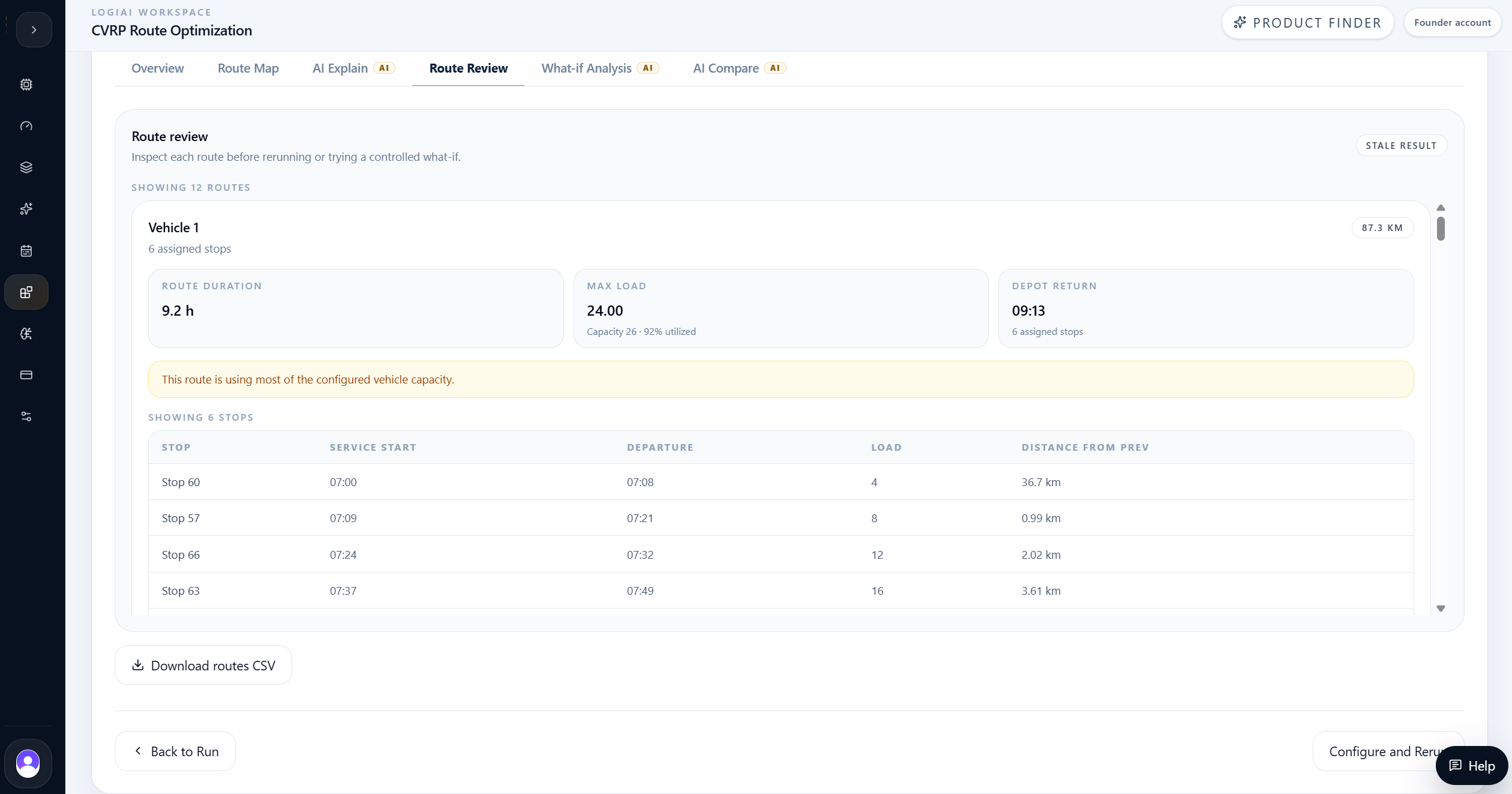
The planning question was whether the current operating footprint was too expensive. A 100% on-time baseline still required 13 vehicles, 13 routes, 762.7 km, and 87.8 aggregate route hours. Several route cards also showed near-capacity loads, which meant the fleet policy was doing real work.
The team needed a controlled branch that did not relax service commitments, remove customers, or change demand. The What-if had to test a practical logistics decision: a more central dispatch point plus slightly higher vehicle capacity.
The optimization model had to preserve:
- All 76 delivery stops had to remain served.
- Time windows were hard constraints, not soft preferences.
- The baseline depot was geographically west of many stop clusters.
- Vehicle count and capacity directly affected route consolidation.
- Route duration included travel, service time, waiting, and depot return.
- The comparison needed to preserve 100% on-time service while reducing route burden.
Scenario setup
LogiAI staged the depot, stops, demand, service time, and delivery windows.
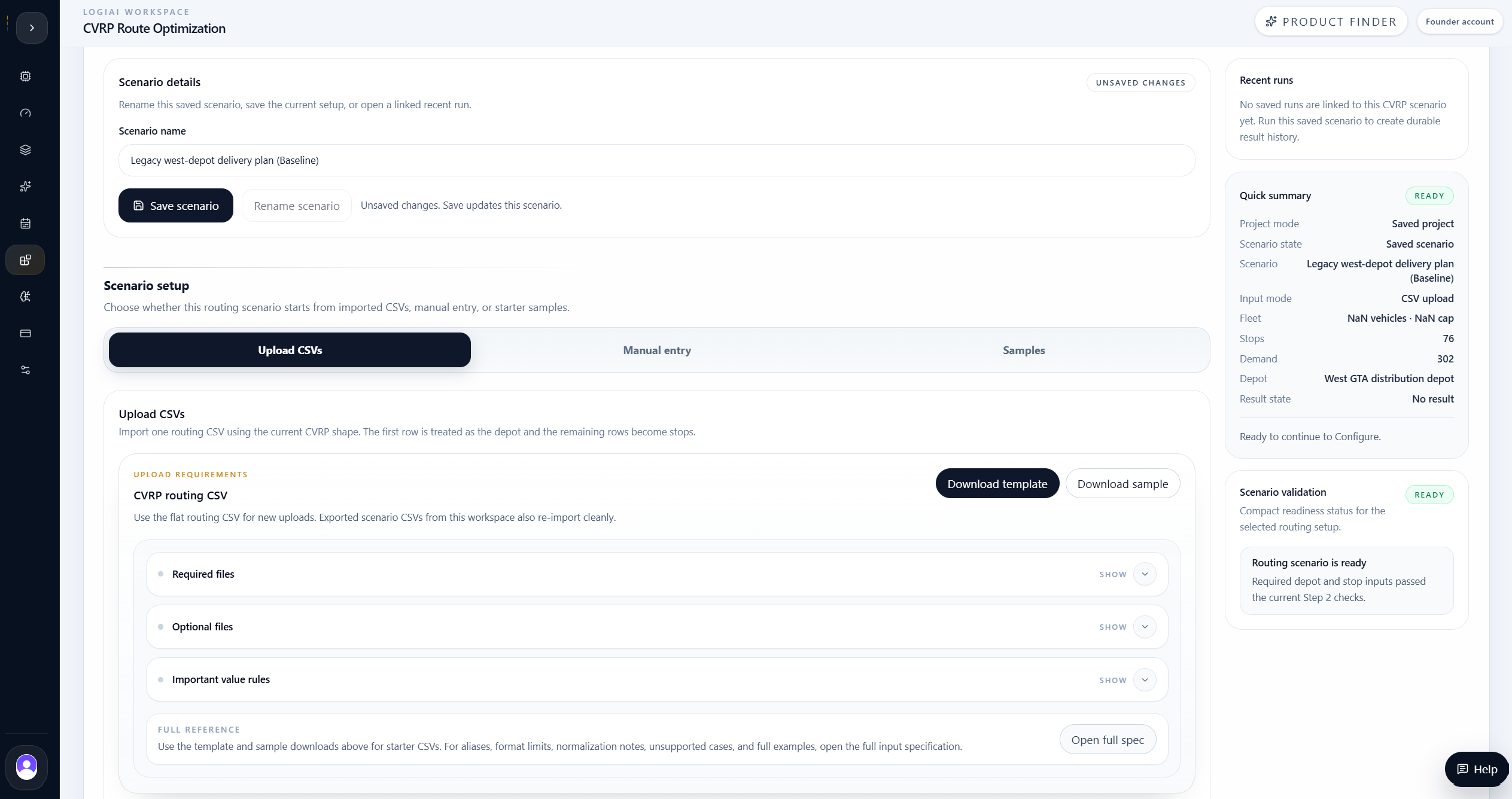
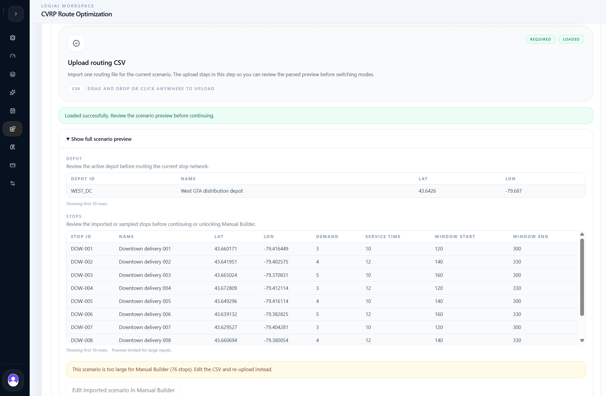
The team uploaded a single routing CSV into LogiAI. The first row represented the depot, and the remaining rows represented the delivery stops.
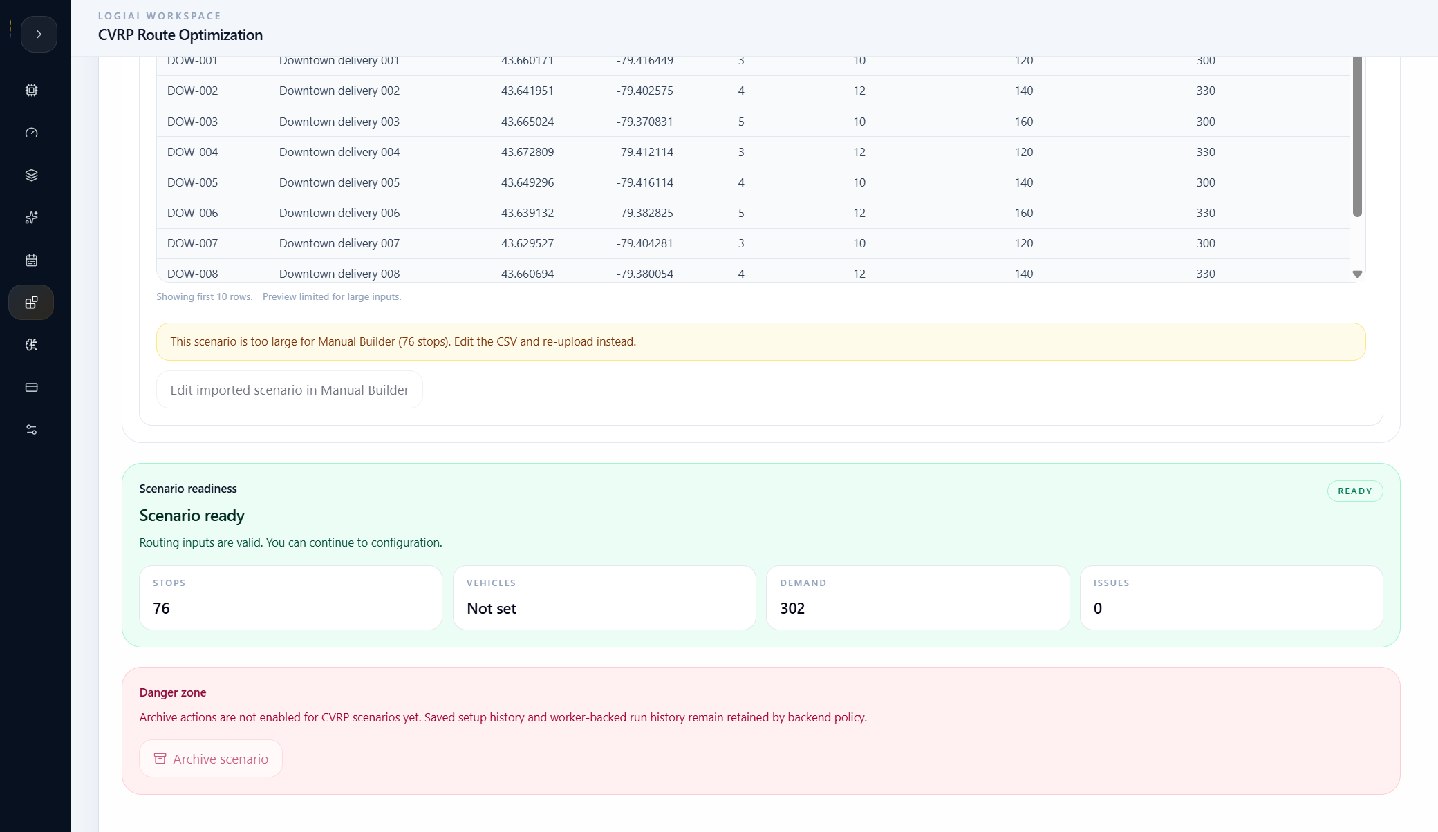
The scenario used 76 customer stops, 302 total demand units, service times per stop, and delivery windows for every customer. The data was large enough to make route structure visible without turning the page into a toy example.
The workspace preview helped confirm the stop records, demand values, service times, and delivery windows before the optimizer was run.
Uploaded routing scope
- 76 stop records plus one depot row.
- 302 total demand units.
- Seven geographic delivery clusters across the GTA.
- Stop-level service times.
- Stop-level time windows in minutes from scenario start.
- Latitude and longitude coordinates for depot and customers.
Configuration
The baseline used balanced routing with tight fleet capacity.
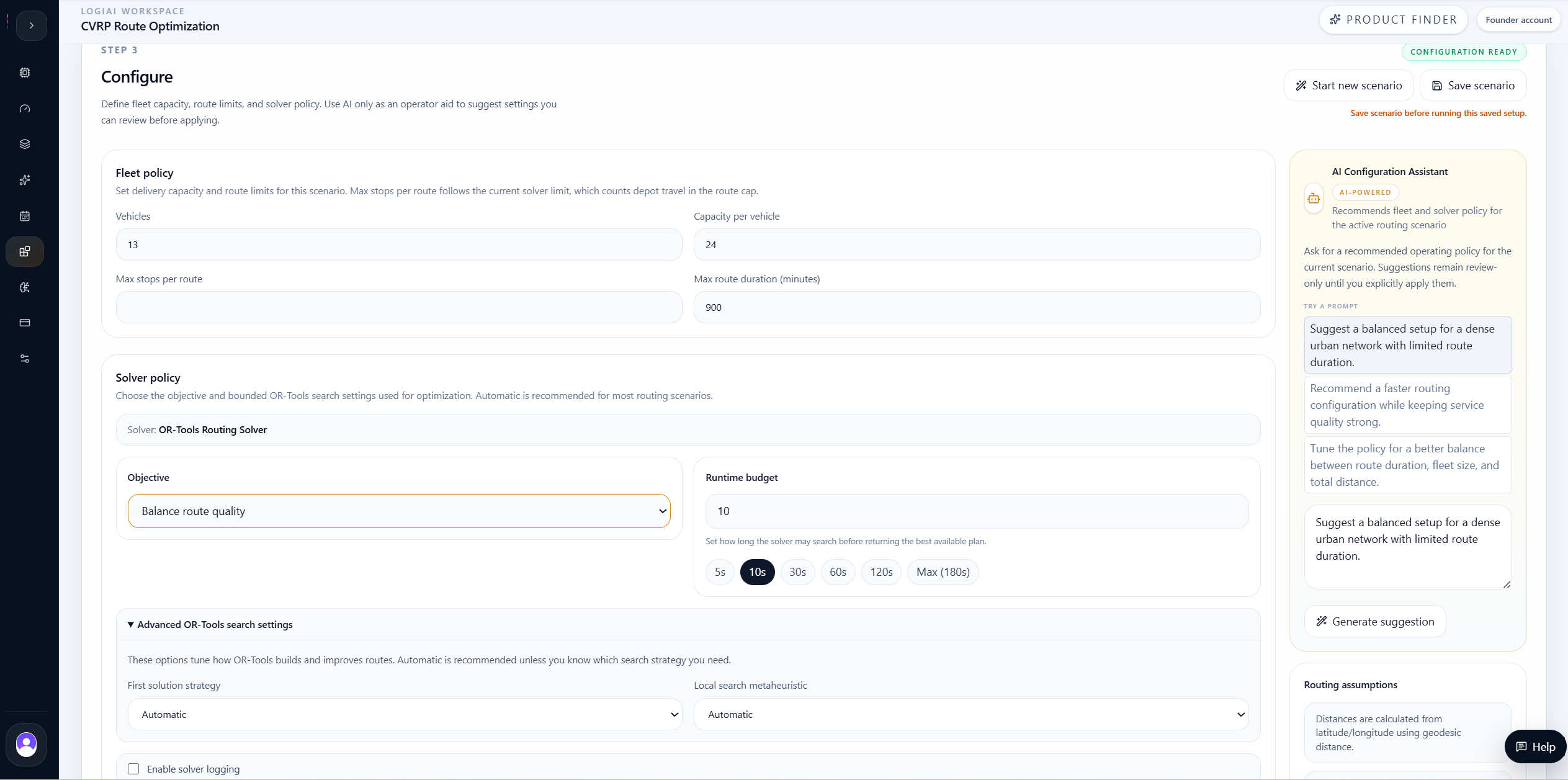
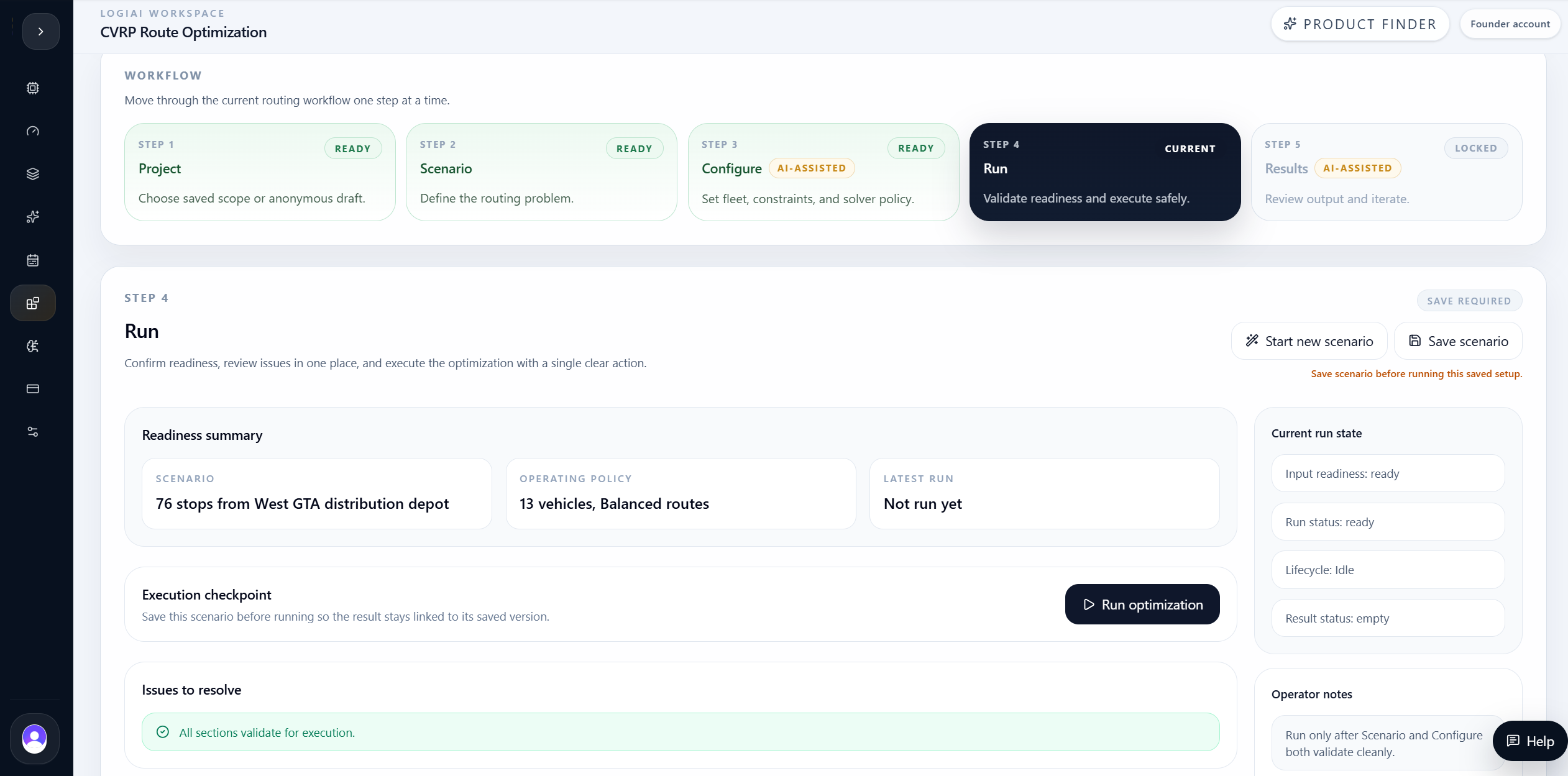
The baseline used the balanced routing objective, 13 vehicles, 24-unit capacity per vehicle, no max-stops-per-route cap, and a 900-minute maximum route duration.
Advanced solver settings stayed automatic and solver logging remained off. That kept the case focused on the routing policy decision, not manual solver tuning.
The configuration also kept the runtime at 10 seconds. The result therefore reflects a normal product workflow: upload the routing scenario, configure fleet policy, run the solver, and compare a controlled branch.
Baseline configuration
- Balanced routes objective.
- 13 baseline vehicles.
- 24-unit baseline capacity per vehicle.
- 900-minute maximum route duration.
- No maximum-stops-per-route cap.
- Automatic first-solution and local-search settings.
- Solver logging off.
Optimization model
The run converted the routing CSV into a constrained vehicle-routing solve.
LogiAI translated the scenario into a CVRP solve with capacity, route-duration, service-time, and hard time-window constraints.
The run step made the model auditable before execution. The team could confirm the depot, stop count, fleet policy, objective, and solver runtime before asking the backend to optimize.
Because the model preserved hard time windows, a feasible result meant every stop could be served inside its requested delivery window.
Optimization model considered
- Each stop must be assigned to a route.
- Vehicle load cannot exceed configured capacity.
- Service starts must respect each stop time window.
- Route duration includes travel, service, time-window waiting, and return to depot.
- The balanced objective evaluates route quality rather than only total distance.
- The solver can use fewer vehicles only when capacity and timing remain feasible.
Baseline evidence
The baseline was feasible, on time, and still expensive.
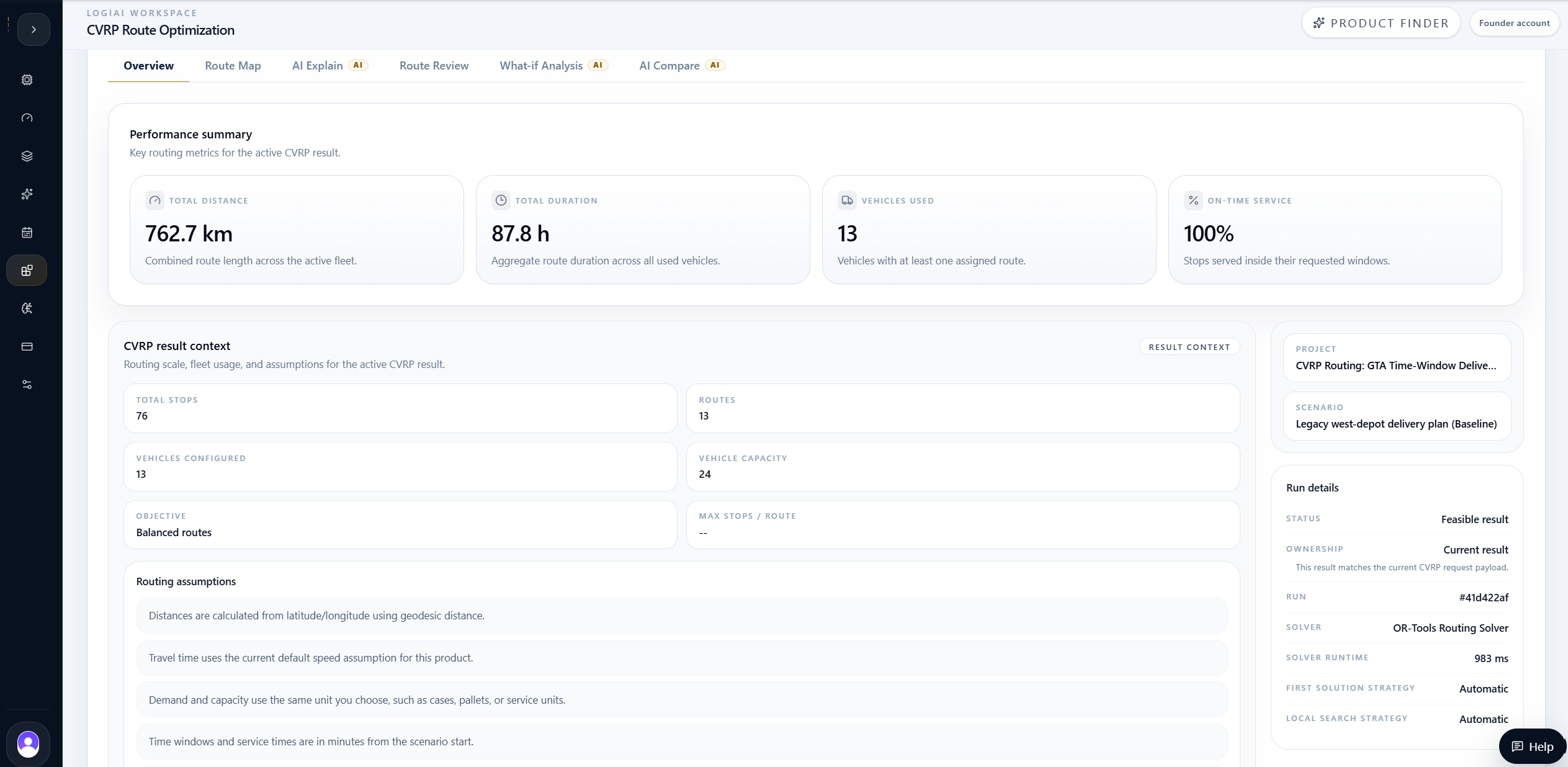
The baseline produced a feasible routing plan with 100% on-time service. That is important, but it is not the same as an optimal operating footprint.
The plan required 13 vehicles and 13 routes to serve the 76 stops. It accumulated 762.7 km of total distance and 87.8 hours of aggregate route duration.
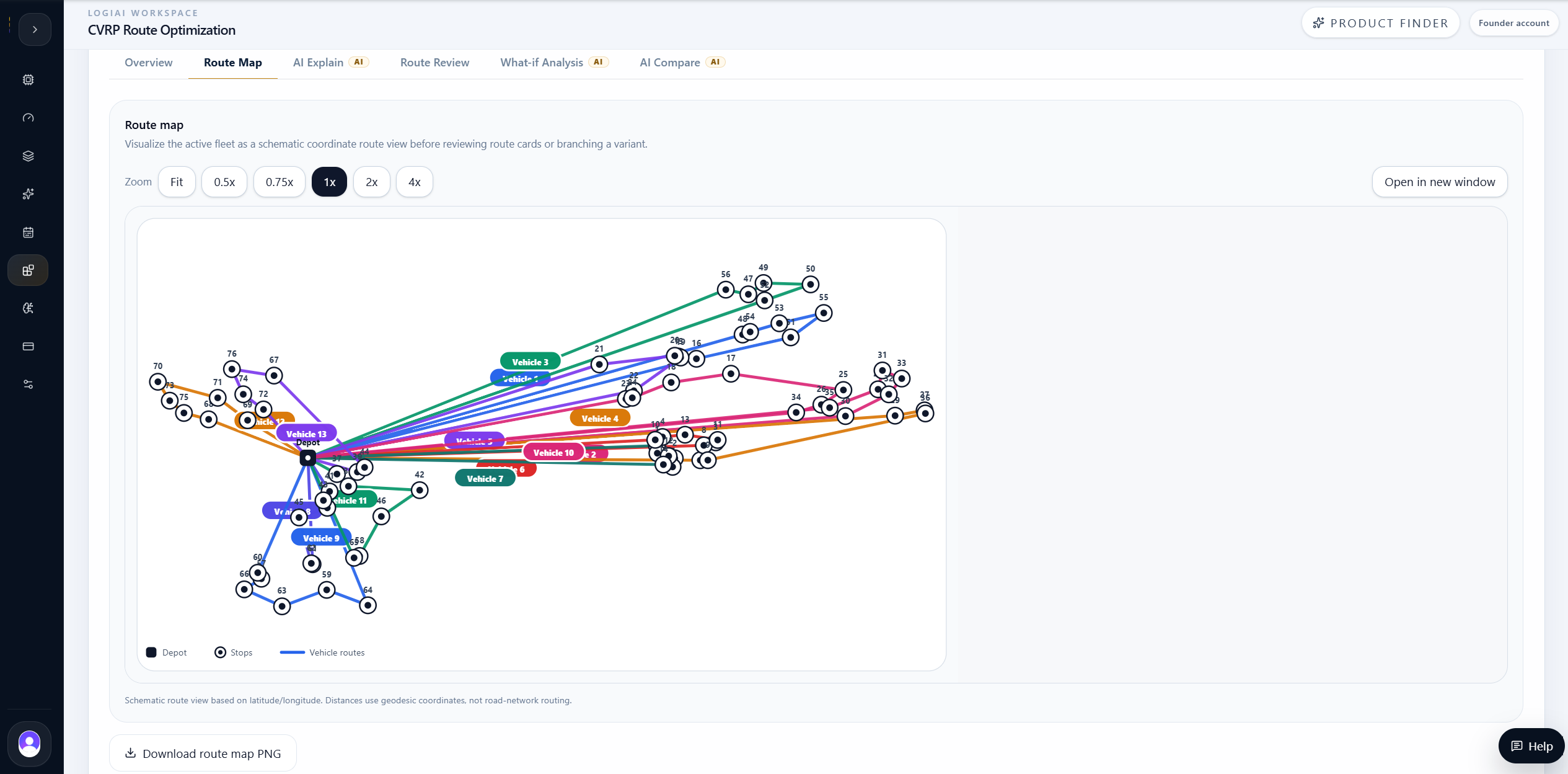
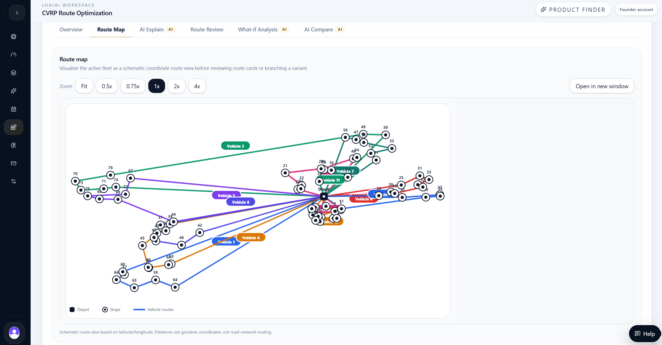
Those numbers made the case useful. The route plan protected every appointment window, but the route map and route review showed the cost of doing so from the legacy west-depot location.
| Metric | Baseline |
|---|---|
| Total stops | 76 |
| Routes | 13 |
| Vehicles configured | 13 |
| Vehicle capacity | 24 |
| Total distance | 762.7 km |
| Total duration | 87.8 h |
| On-time service | 100% |
| Solver runtime | 983 ms |
AI Explain
AI Explain diagnosed route burden instead of pretending lateness was the issue.
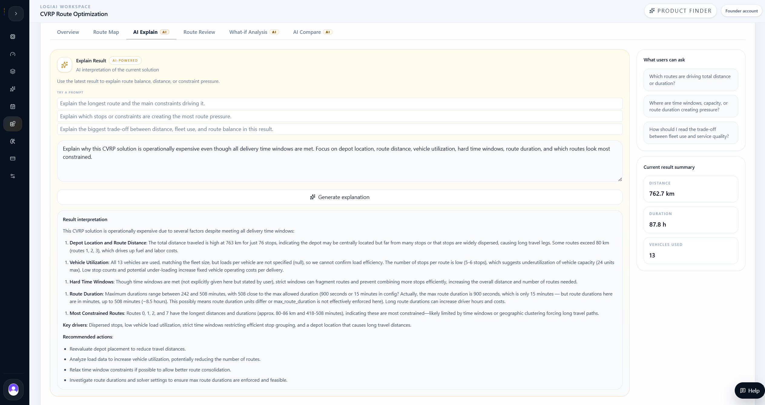
AI Explain helped keep the interpretation honest. Since the time windows are hard, the right diagnosis is not that customers are late. The diagnosis is that the current plan is expensive even while it keeps every customer promise.
The explanation highlighted depot location, route distance, vehicle utilization, hard time windows, and route-duration pressure as the practical reasons the baseline deserved a What-if test.
That led to a precise scenario: do not relax delivery windows, do not remove stops, and do not change demand. Instead, test whether a central micro-hub and modest capacity change can reduce route burden.
What-if Analysis
The branch tested a Midtown micro-hub and fleet consolidation.
What the branch changed
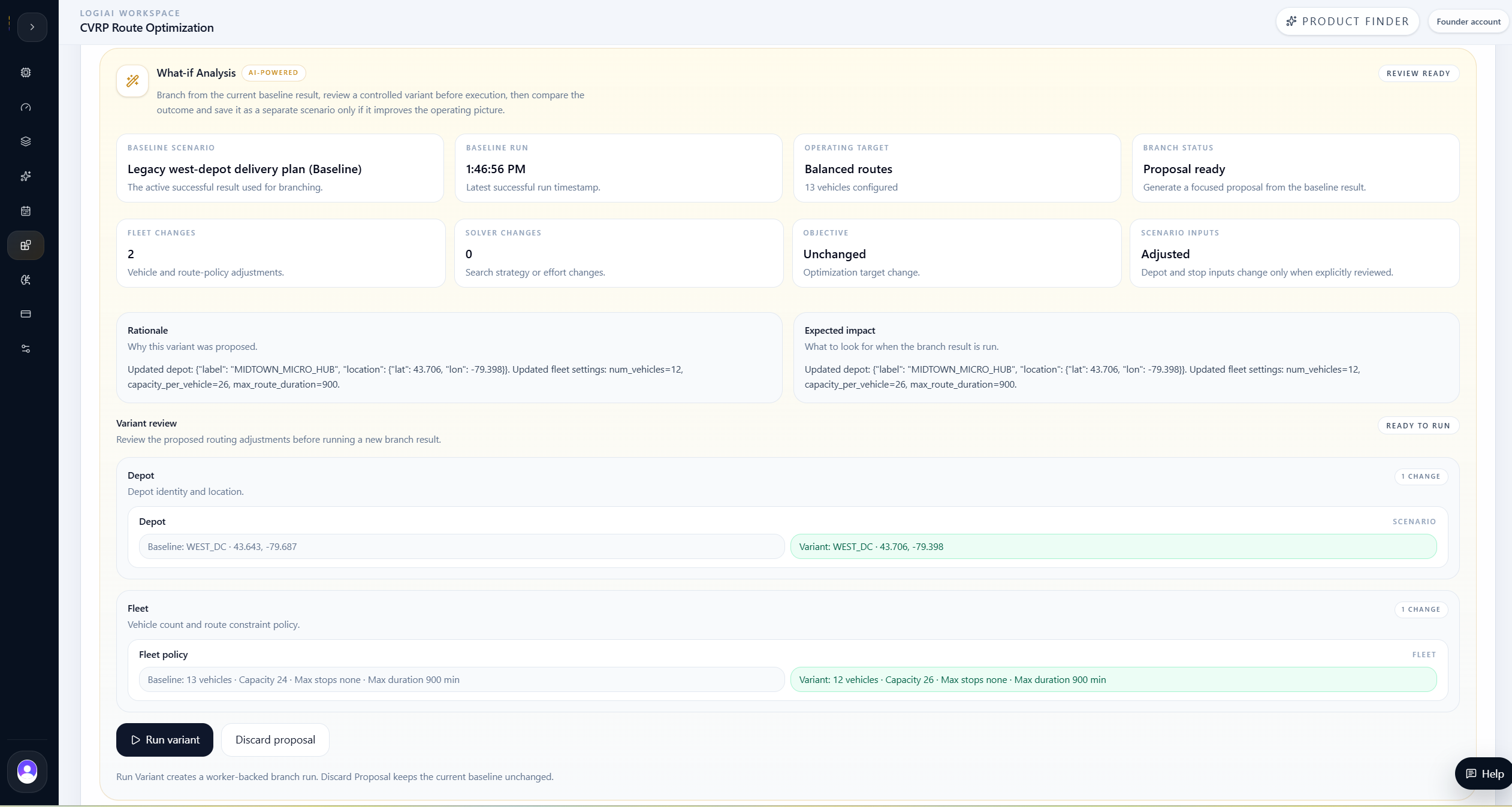
- Moved dispatch to MIDTOWN_MICRO_HUB.
- Changed vehicles from 13 to 12.
- Changed capacity per vehicle from 24 to 26.
- Kept the same 76 stops and time windows.
- Kept max route duration at 900 minutes.
- Kept balanced objective and automatic solver settings.
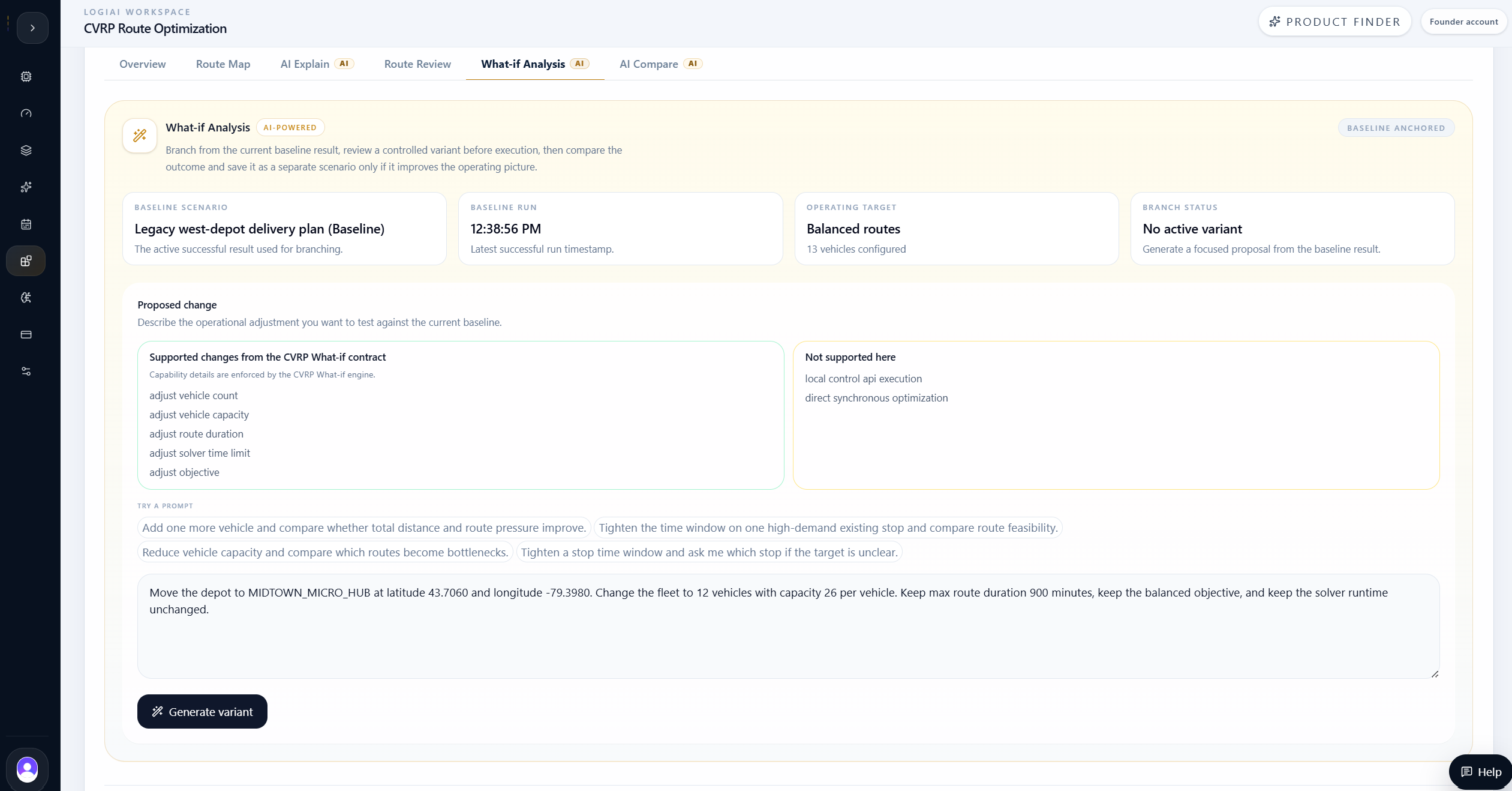
The What-if branch moved dispatch from WEST_DC to MIDTOWN_MICRO_HUB at latitude 43.7060 and longitude -79.3980.
The same branch changed the fleet from 13 vehicles at 24 capacity to 12 vehicles at 26 capacity. Max route duration stayed at 900 minutes, the balanced objective stayed unchanged, and the same 76 time-windowed stops remained in scope.
This made the branch operationally meaningful. It tested a depot and fleet-policy decision, not a cosmetic parameter change.
Midtown micro-hub branch result
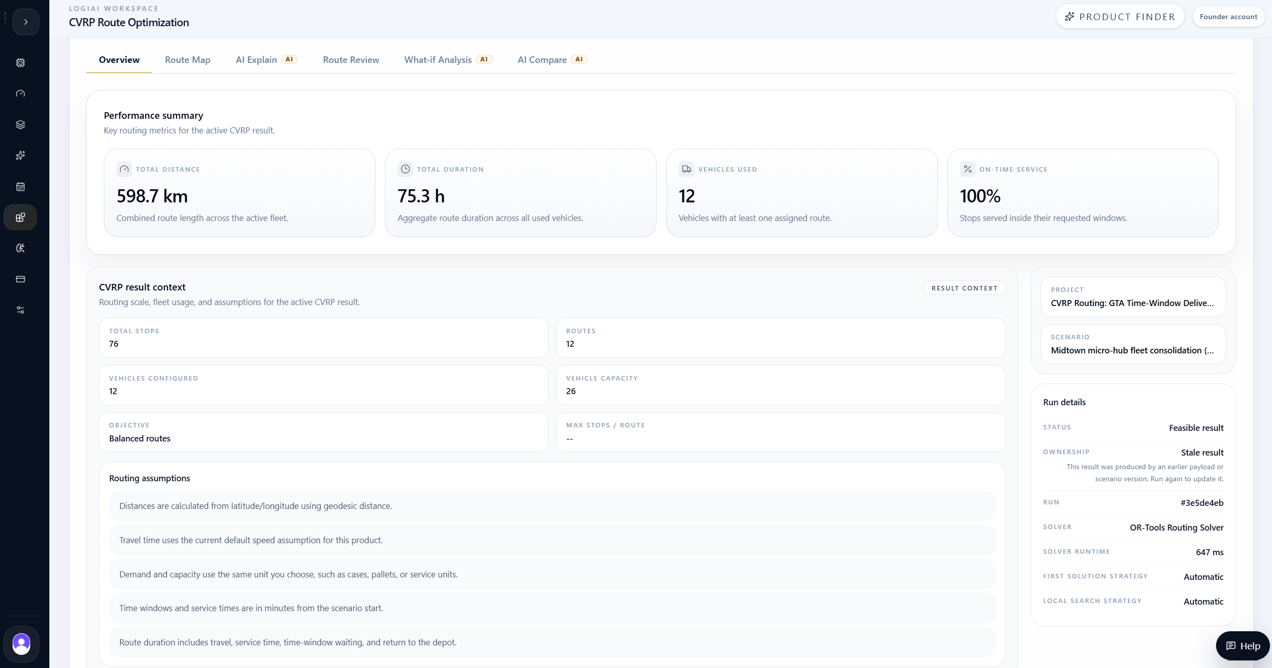
The branch completed as a stronger routing plan. It kept 100% on-time service, served the same 76 stops, and reduced the fleet footprint from 13 routes to 12.
The result was not just a lower-distance map. The route-duration burden fell from 87.8 hours to 75.3 hours, which means the micro-hub and capacity change reduced the operating effort needed to keep the same customer promise.
| Metric | Baseline | Midtown branch |
|---|---|---|
| Total distance | 762.7 km | 598.7 km |
| Total duration | 87.8 h | 75.3 h |
| Vehicles used | 13 | 12 |
| Routes used | 13 | 12 |
| On-time service | 100% | 100% |
AI Compare
AI Compare showed why the Midtown branch was the stronger scenario.
After saving the Midtown micro-hub branch, the team used AI Compare to evaluate the saved baseline against the saved variant.
The comparison was intentionally narrow: Baseline was the legacy WEST_DC plan with 13 vehicles at 24 capacity, and the variant was the MIDTOWN_MICRO_HUB plan with 12 vehicles at 26 capacity. The stop list, delivery windows, balanced objective, 900-minute route-duration policy, and 10-second solve budget stayed the same.
Baseline scenario
Legacy WEST_DC delivery plan with 13 vehicles, 24-unit capacity, balanced routes, 76 stops, hard time windows, and 900-minute route-duration policy.
Midtown branch
MIDTOWN_MICRO_HUB dispatch with 12 vehicles, 26-unit capacity, the same customer stops, the same windows, and the same routing objective.
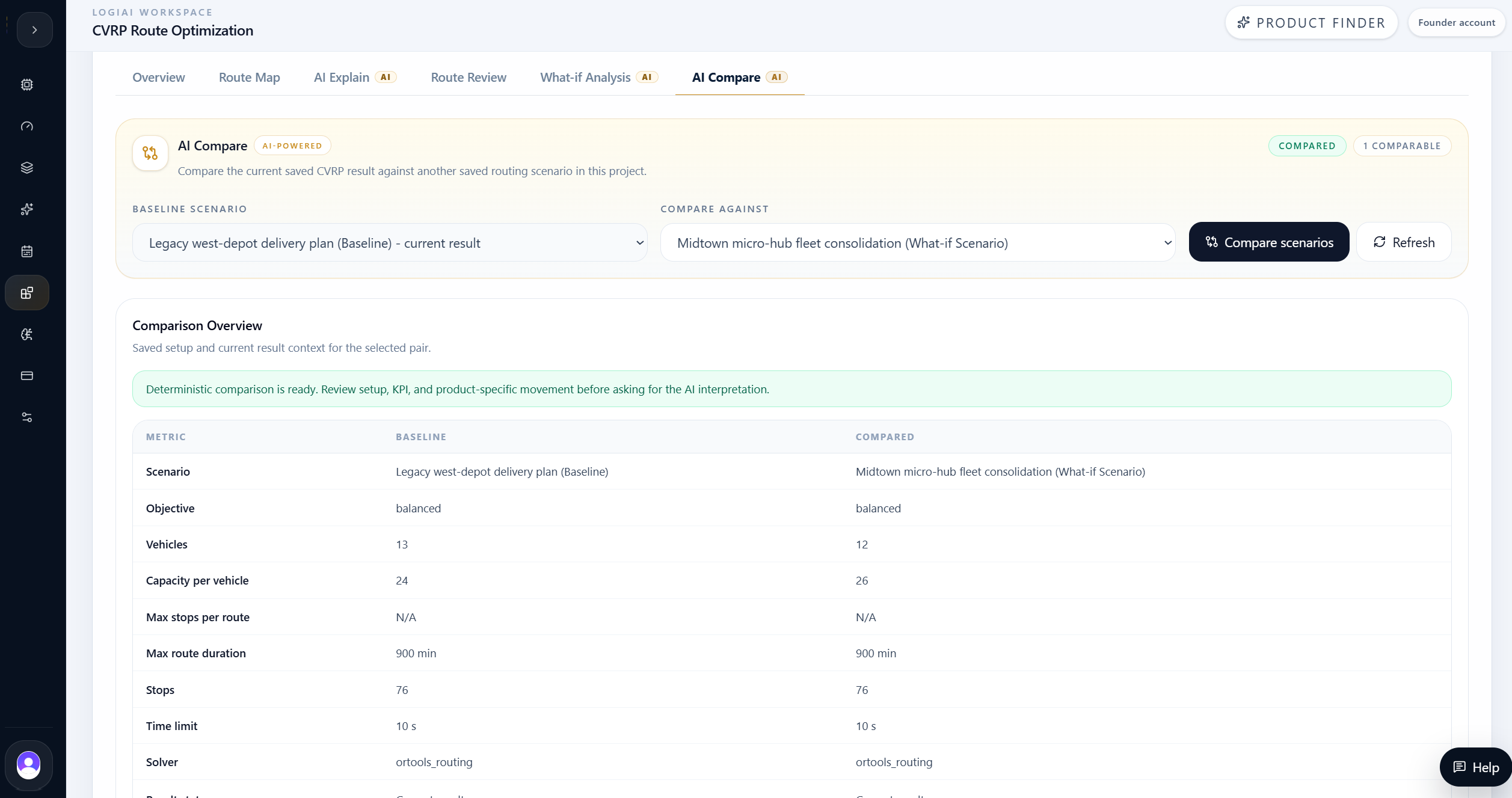
That made the result easy to trust. The variant reduced total distance by 164.0 km and total duration by 12.5 hours while using one fewer vehicle. It did this without losing the 100% on-time service level or dropping any of the 76 stops.
AI Compare also clarified the kind of decision being made. This was not a service-level trade-off where fewer vehicles created lateness. It was a network-design improvement: the dispatch point moved closer to the demand center, and capacity increased enough to consolidate one route.
The baseline remained feasible, so the comparison did not argue that the old plan was broken. It argued that the old plan was unnecessarily expensive for the same delivery promise.
Distance
Baseline: 762.7 km
Variant: 598.7 km
-164 km
Duration
Baseline: 87.8 h
Variant: 75.3 h
-12.5 h
Vehicles
Baseline: 13
Variant: 12
-1
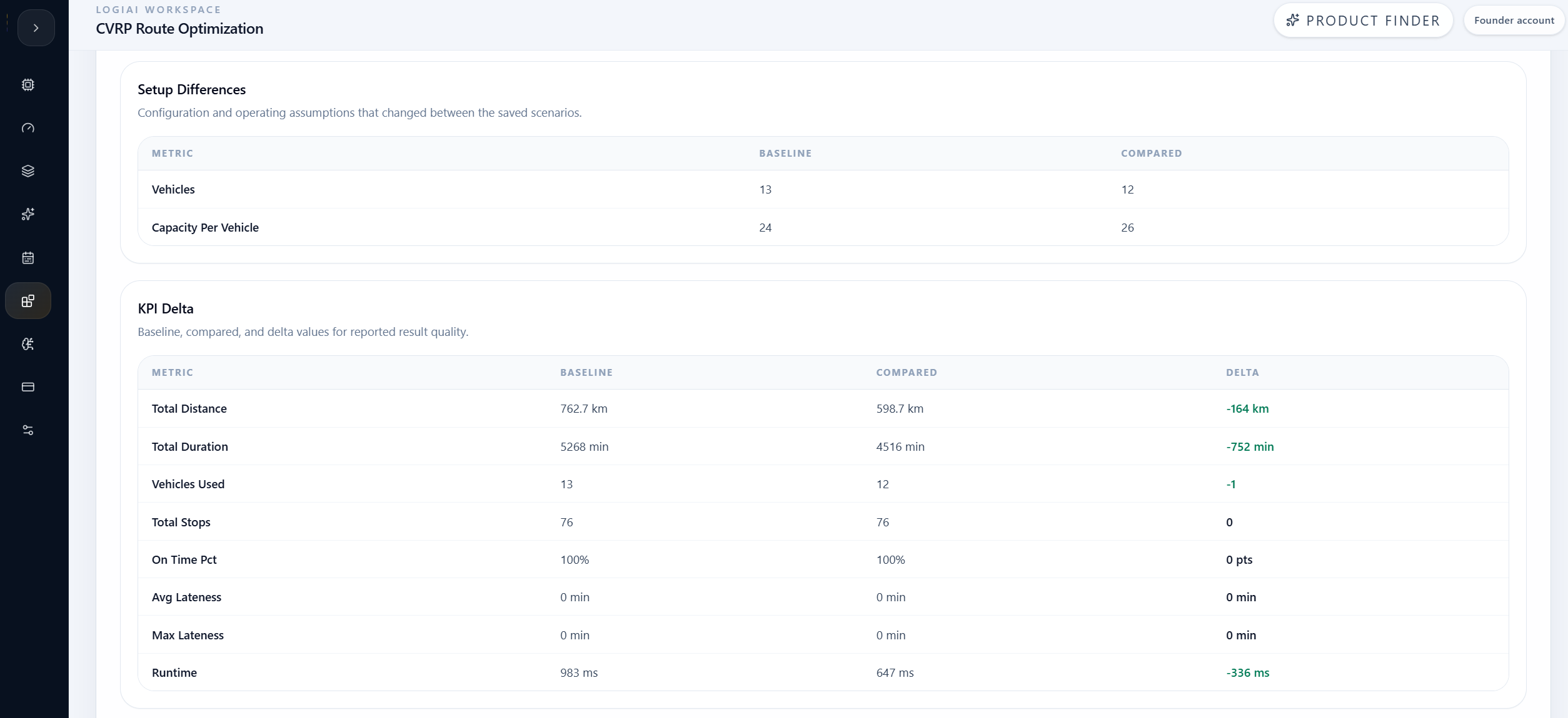
| Metric | Baseline | Midtown branch | Delta |
|---|---|---|---|
| Total distance | 762.7 km | 598.7 km | -164 km |
| Total duration | 5268 min | 4516 min | -752 min |
| Vehicles used | 13 | 12 | -1 |
| Total stops | 76 | 76 | No change |
| On-time service | 100% | 100% | No change |
| Average lateness | 0 min | 0 min | No change |
| Max lateness | 0 min | 0 min | No change |
| Runtime | 983 ms | 647 ms | -336 ms |
What AI Summary added
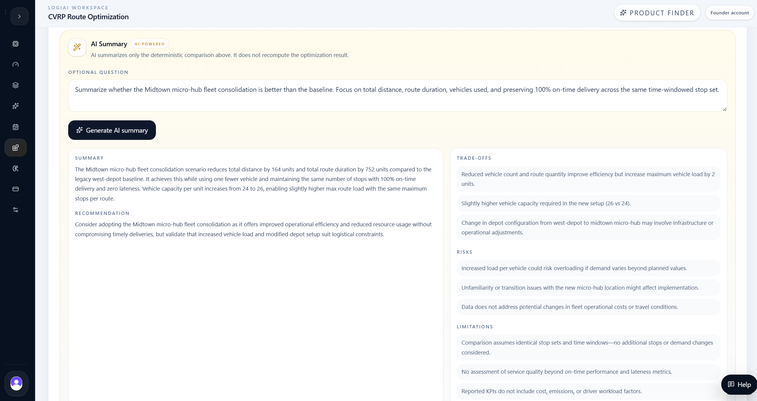
The AI Summary turned the deterministic KPI movement into an operating recommendation. It framed the Midtown branch as the stronger candidate because it lowered distance, duration, and vehicle count while preserving the same hard delivery-window performance.
The summary also made the adoption caveat clear: before changing the real operation, the team should validate whether the Midtown micro-hub is available, whether the 26-unit vehicles are realistic, and whether depot operating costs still support the savings.
Decision
The better plan preserved service quality while reducing the route footprint.
The team selected the Midtown micro-hub fleet consolidation as the stronger scenario to review.
The baseline was service-feasible, but expensive. The variant protected the same time-window promise while reducing distance, route duration, and vehicle count.
The final recommendation was not to add random fleet capacity. It was to move dispatch closer to the demand center and use slightly higher-capacity vehicles so the operation could consolidate routes without sacrificing on-time delivery.
For routing teams, that is the practical value of LogiAI CVRP: it can validate a feasible baseline, explain why it still costs too much, test a realistic operating policy, and compare the result before changing the network.
A 100% on-time route plan can still be operationally expensive.
Hard time windows make the customer promise explicit during optimization.
AI Explain helped shift the question from lateness to route burden and depot footprint.
What-if Analysis tested one realistic logistics decision across depot and fleet policy.
AI Compare showed the exact KPI movement before the team adopted the branch.