
Executive Summary
SchedAI helped the team choose a stronger production schedule before execution.
A precision manufacturing team needed to evaluate a flexible job shop schedule before releasing it to production. The plan involved 12 jobs, around 60 operations, 7 machines, due dates, priorities, setup logic, release times, and maintenance windows.
SchedAI modeled the production environment, generated a feasible baseline, explained the schedule, tested what-if scenarios, and compared alternatives before the team made an operational decision.
The strongest result came from increasing solver runtime from 60 seconds to 120 seconds. That scenario reduced makespan from 181.0 to 168.0, weighted tardiness from 563.0 to 495.0, and max machine idle time from 121.0 to 100.0.
Makespan
181.0 to 168.0
Weighted tardiness
563.0 to 495.0
Max machine idle
121.0 to 100.0
Core capabilities exercised
- Flexible job shop scheduling with ordered operations and eligible machine alternatives.
- Machine availability, processing times, setup times, release times, and maintenance windows.
- Due-date and priority-aware objectives, including weighted tardiness.
- Solver runtime tuning for deeper optimization when the baseline is feasible but still weak.
- Gantt-style timeline review for machine lanes, gaps, bottlenecks, and assignment movement.
- What-if scenario branches for testing operational changes before execution.
- AI Explain and AI Compare for interpreting schedule quality, trade-offs, and final decisions.
Factory Context
A real flexible job shop planning problem.
A mid-sized precision manufacturing company produces customized industrial components in small and varied batches. Each customer order moves through multiple production operations, and many operations can be processed on more than one eligible machine.
This flexibility gives the factory more scheduling options, but it also creates a complex planning challenge. The team must decide which job should run first, which machine should handle each operation, how to manage setup transitions, and how to avoid conflicts with planned maintenance windows.
SchedAI was used to model this flexible job shop environment, generate a feasible baseline schedule, explain the result, and test an improved scenario before execution.
The factory manages multiple customer orders at the same time. Each order must pass through a defined sequence of operations before it can be completed.
The production floor includes seven machines with overlapping capabilities. Some operations can be processed on more than one machine, but each machine has different processing times, availability, setup requirements, and maintenance interruptions.
This means the schedule cannot be created by simply arranging jobs in order. Every scheduling decision affects the next one. Assigning one operation to a specific machine may reduce waiting time for one job, but create congestion for another. Running jobs in the wrong sequence may increase setup time or push important orders beyond their due dates.
As order variety increases, manual planning becomes harder to control. A small change in machine assignment, operation sequence, or job priority can affect the full production timeline.
SchedAI was used to help the planning team evaluate these connected decisions together and produce a schedule that respects real production constraints.
Scheduling Challenge
The schedule had to respect operational constraints, not just fill a calendar.
The main challenge was to build a feasible production schedule in a flexible job shop environment.
The team needed to reduce delays without creating an unrealistic schedule.
Without optimization support, the team risked creating schedules that looked practical at first, but later caused delayed jobs, machine idle time, poor workload balance, unnecessary setup changes, or conflicts with planned maintenance.
The factory needed more than a visual calendar. It needed a system that could evaluate many scheduling decisions together and show whether a schedule was truly feasible before production started.
Constraints considered
- Each job had a required operation sequence.
- Each operation could run only on eligible machines.
- Machines had different processing times.
- Setup times affected transitions between jobs.
- Some jobs were available only after their release times.
- Jobs had due dates and priorities.
- Machines had planned maintenance windows.
Why SchedAI was needed
SchedAI was needed because the problem involved more than arranging tasks on a timeline.
The factory needed a scheduling tool that could reason through machine alternatives, operation sequences, setup times, release times, due dates, priorities, and maintenance windows together.
Instead of testing machine assignments and job sequences manually, the planning team could use SchedAI to evaluate many possible combinations and generate a schedule that respected the real constraints of the production floor.
The value of SchedAI in this case was not only in generating a schedule. It also helped the team understand the result. The team could see how jobs were assigned, where machine time was used, where delays appeared, and how changes in solver settings could affect schedule performance.
By combining optimization, AI-supported explanation, and what-if comparison, SchedAI helped the planning team move from manual trial-and-error planning to a more structured scheduling process.
Method: Input Setup
The team first modeled the production environment.
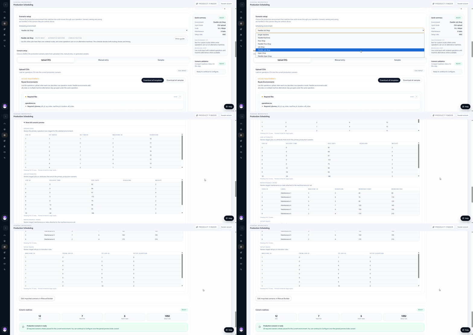
The first step was to define the production environment as a flexible job shop.
The factory provided the scheduling data needed to model the problem. The dataset included 12 production jobs, around 60 operations, and 7 machines.
After this data was entered, SchedAI had enough information to represent how work moved through the factory and which constraints had to be respected.
Input setup included
- Jobs to be scheduled
- Operation sequence for each job
- Available machines and eligible machine alternatives
- Processing times and setup times
- Release times, due dates, and job priorities
- Planned machine maintenance windows
Method: Configuration
Configuration adapted to the scenario data.
After the input data was prepared, the team moved to the configuration step.
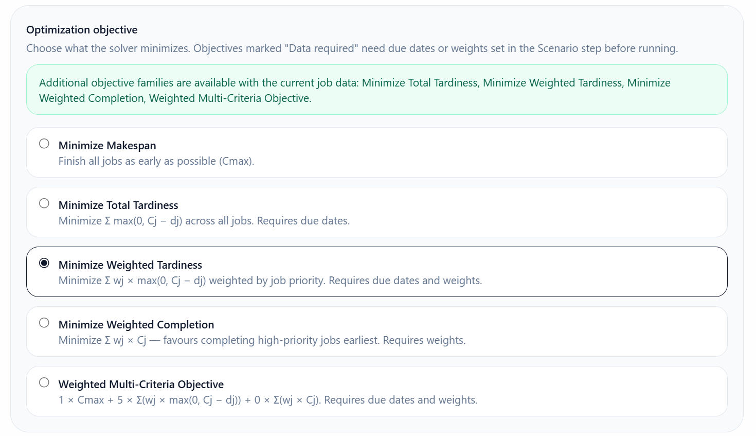
SchedAI allowed the team to choose the solver, define the solver time limit, and select the scheduling objective.
For the baseline run, the solver time limit was set to 60 seconds. The objective focused on weighted tardiness, which means the schedule aimed to reduce lateness while giving more importance to higher-priority jobs.
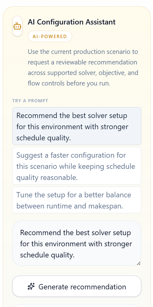
AI Configure helped guide the setup by recommending practical optimization settings based on the structure of the flexible job shop scenario.
This allowed the planning team to configure the scheduling run without needing to write optimization code, formulate mathematical constraints, or tune solver parameters manually.
- Smart objective options appear when due dates and weights make tardiness objectives available.
- The planner keeps solver, runtime, objective, and flow policy visible before the run.
- The AI Configuration Assistant helps when solver or objective settings need explanation.
Method: Run Optimization
SchedAI translated the inputs into a constrained scheduling model.
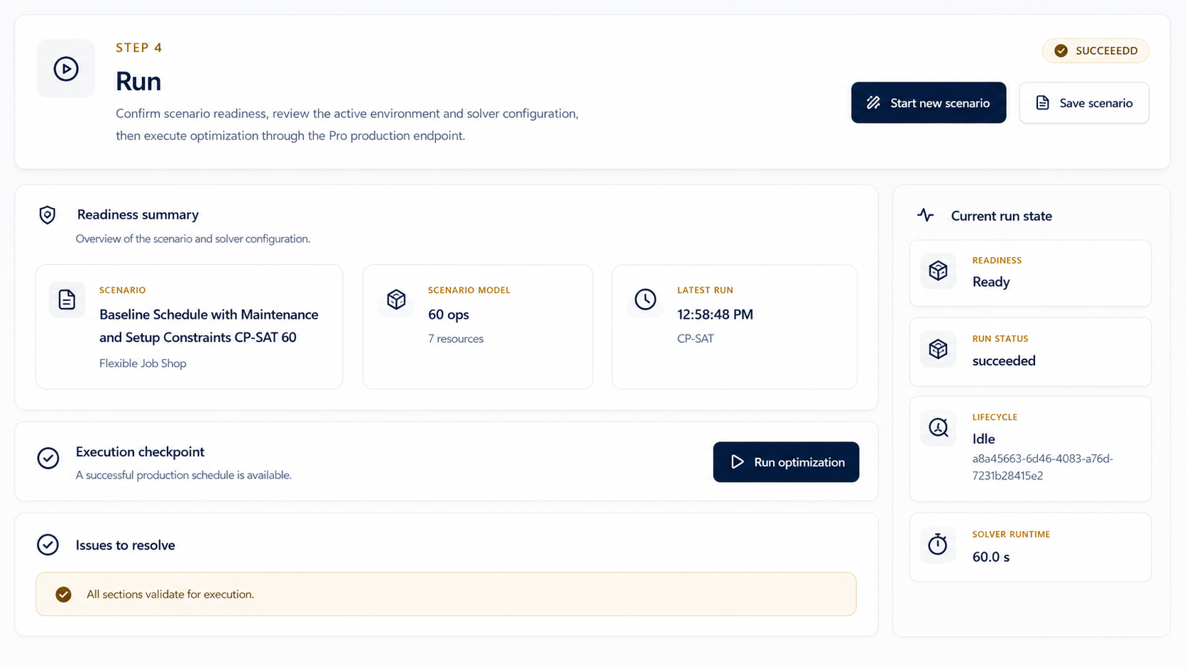
After configuration, SchedAI translated the input data and selected settings into a constrained scheduling model.
The result was a feasible baseline schedule that assigned operations to eligible machines while respecting the main operational constraints.
Optimization engine considered
- Job operation sequences
- Eligible machine alternatives
- Machine availability
- Processing times
- Setup times
- Release times
- Due dates
- Job priorities
- Maintenance windows
Baseline Evidence
SchedAI generated a feasible schedule, then exposed its limits.
| Baseline KPI | Value |
|---|---|
| Makespan | 181.0 |
| Weighted tardiness | 563.0 |
| Total tardiness | 264.0 |
| On-time rate | 50.0% |
| Average flow time | 85.5 |
| Machine utilization | 56.7% |
| Max machine idle | 121.0 |
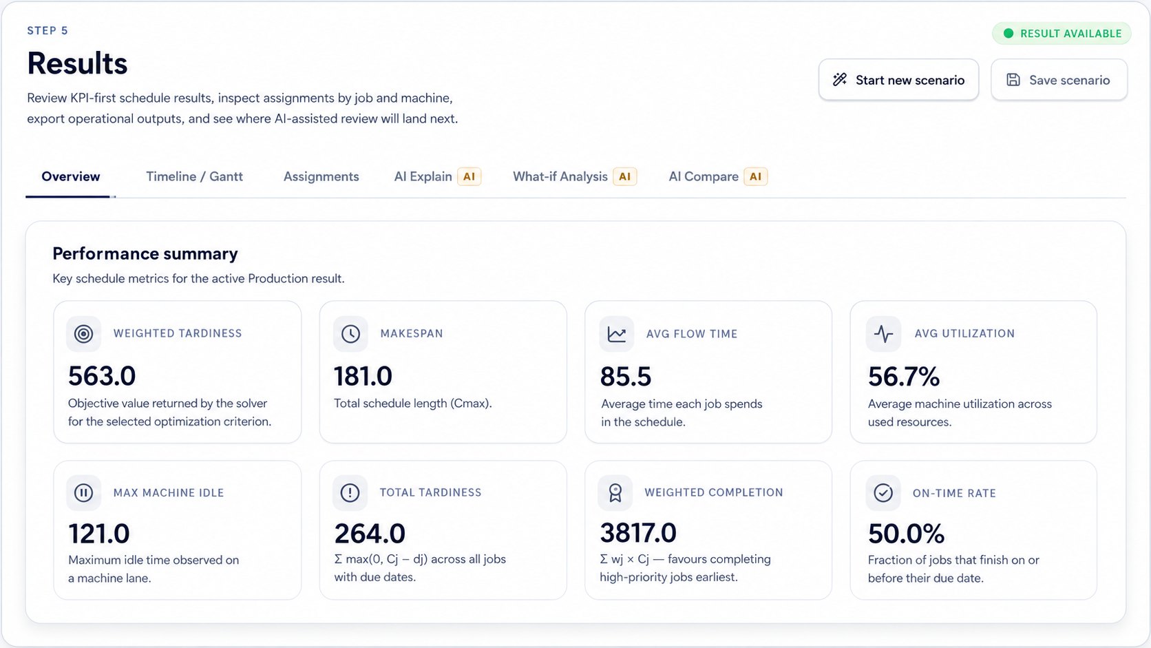
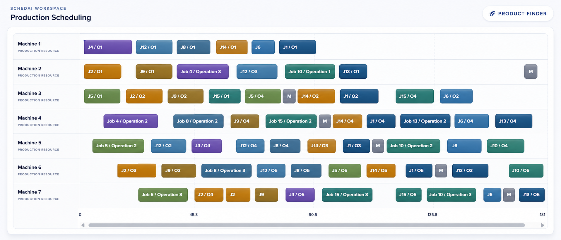
After running the baseline scenario, SchedAI generated a feasible production schedule and displayed the main performance indicators together with a visual Gantt chart.
The baseline KPI results showed that SchedAI was able to generate a feasible production schedule under the given flexible job shop constraints.
The makespan was 181.0, representing the total schedule length from the first operation to the final completion. The result also showed a weighted tardiness of 563.0 and total tardiness of 264.0, which indicated that several jobs finished after their due dates, including higher-priority jobs.
The on-time rate was 50.0%, meaning that half of the jobs were completed on or before their due dates. Average flow time was 85.5, showing that jobs spent a significant amount of time in the production system before completion.
Machine utilization reached 56.7%, while the maximum machine idle time was 121.0. These metrics showed that the baseline schedule was feasible, but there was still room to improve delivery performance, reduce waiting time, and make better use of available machine capacity.
The Gantt chart helped the team see how operations were arranged across the machine lanes. Maintenance blocks showed when machines were unavailable, while empty spaces between operations helped reveal waiting time, idle capacity, or scheduling gaps caused by release times, operation dependencies, setup requirements, or machine availability.
AI Explain
AI Explain turned the baseline into operational insight.
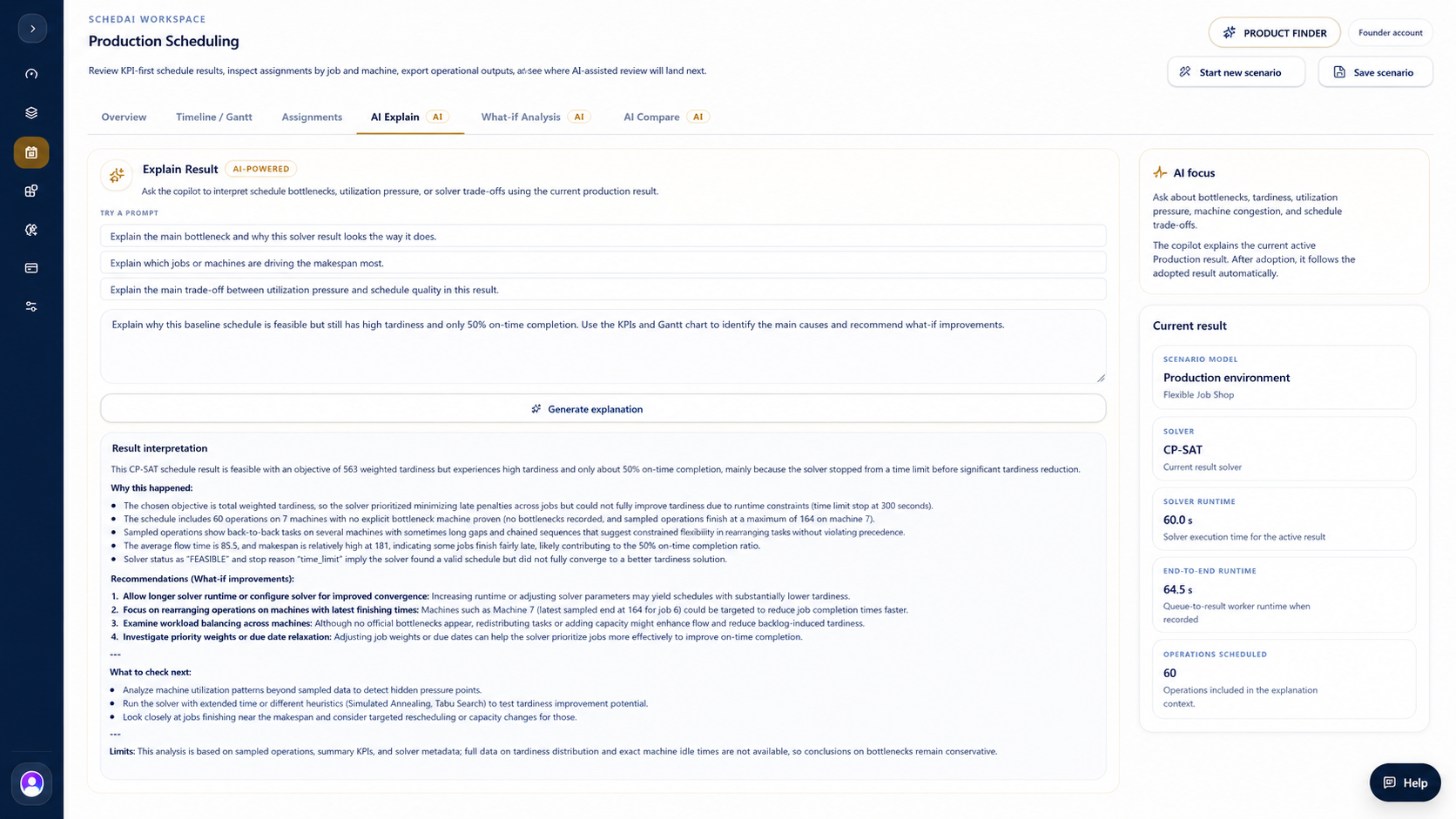
After reviewing the baseline KPIs and Gantt chart, the team used AI Explain to understand why the schedule looked the way it did.
AI Explain showed that the schedule was feasible, but the result still had high tardiness and only 50.0% on-time completion.
The explanation highlighted that the solver was optimizing for weighted tardiness, meaning it was trying to reduce lateness while giving more importance to higher-priority jobs.
However, the scheduling problem was complex. It included around 60 operations, 7 machines, multiple machine alternatives, setup times, release times, due dates, priorities, and maintenance windows.
AI Explain helped the team understand that the result was not caused by one simple issue. The schedule included back-to-back machine assignments, waiting gaps between operations, and some jobs finishing close to the end of the schedule.
These factors contributed to the high tardiness and the 50.0% on-time rate.
AI Explain also suggested a practical next step: give the solver more time to search for better machine assignments and job sequences.
This helped the planning team move from simply looking at numbers to understanding what could be improved and why.
What-if Analysis
The team tested planning decisions before releasing the schedule.
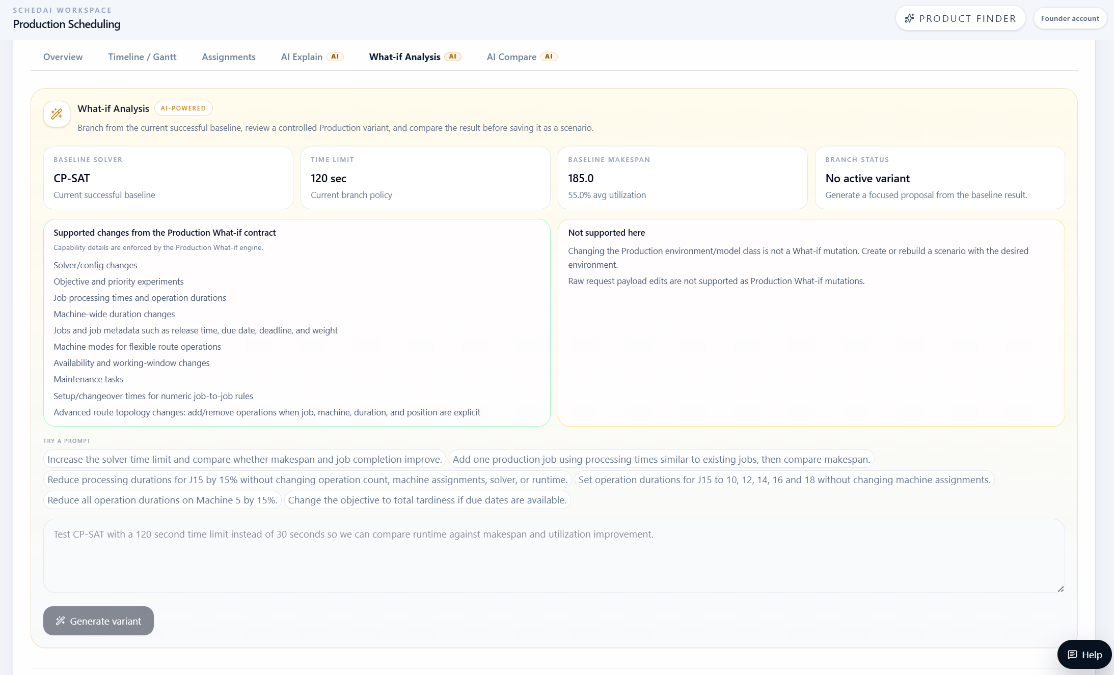
After reviewing the baseline results and the AI Explain output, the team used What-if Analysis to test whether the schedule could be improved before being released to production.
The goal was not to change the production problem itself, but to evaluate possible planning decisions in a controlled way. The team wanted to understand how different changes would affect the schedule before making an operational commitment.
Scenario 1: increasing solver runtime
The first what-if scenario tested a deeper optimization run.
Based on the AI Explain recommendation, the solver time limit was increased from 60 seconds to 120 seconds. This gave SchedAI more time to explore alternative job sequences, machine assignments, and scheduling combinations.
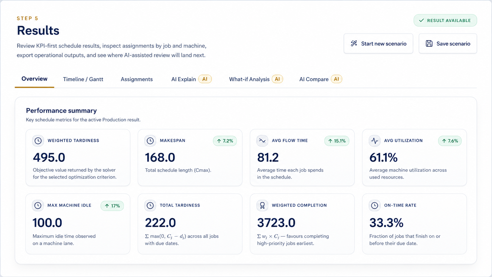
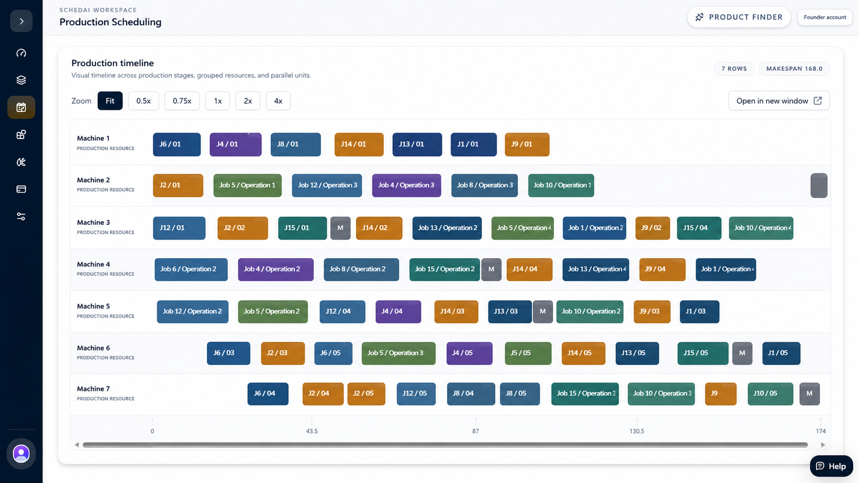
The 120-second scenario produced a stronger schedule than the baseline. Makespan decreased from 181.0 to 168.0. Weighted tardiness decreased from 563.0 to 495.0, and total tardiness decreased from 264.0 to 222.0.
Average flow time improved from 85.5 to 81.2. Average machine utilization increased from 56.7% to 61.1%, and maximum machine idle time decreased from 121.0 to 100.0.
This showed that the original schedule was feasible, but additional optimization time helped SchedAI find a more efficient production plan.
| Metric | 60 sec | 120 sec |
|---|---|---|
| Makespan | 181.0 | 168.0 |
| Weighted tardiness | 563.0 | 495.0 |
| Total tardiness | 264.0 | 222.0 |
| Average flow time | 85.5 | 81.2 |
| Average utilization | 56.7% | 61.1% |
| Max machine idle | 121.0 | 100.0 |
Scenario 2: shifting Machine 6 maintenance
After reviewing the improved schedule, the maintenance team wanted to test whether adjusting one planned maintenance window could further improve production flow.
The team tested a realistic operational question: if the maintenance window on Machine 6 was moved slightly later, would the schedule gain more useful production capacity before the machine became unavailable?
Using What-if Analysis, the maintenance window on Machine 6 was shifted by 10 time units, from 120-165 to 130-175.
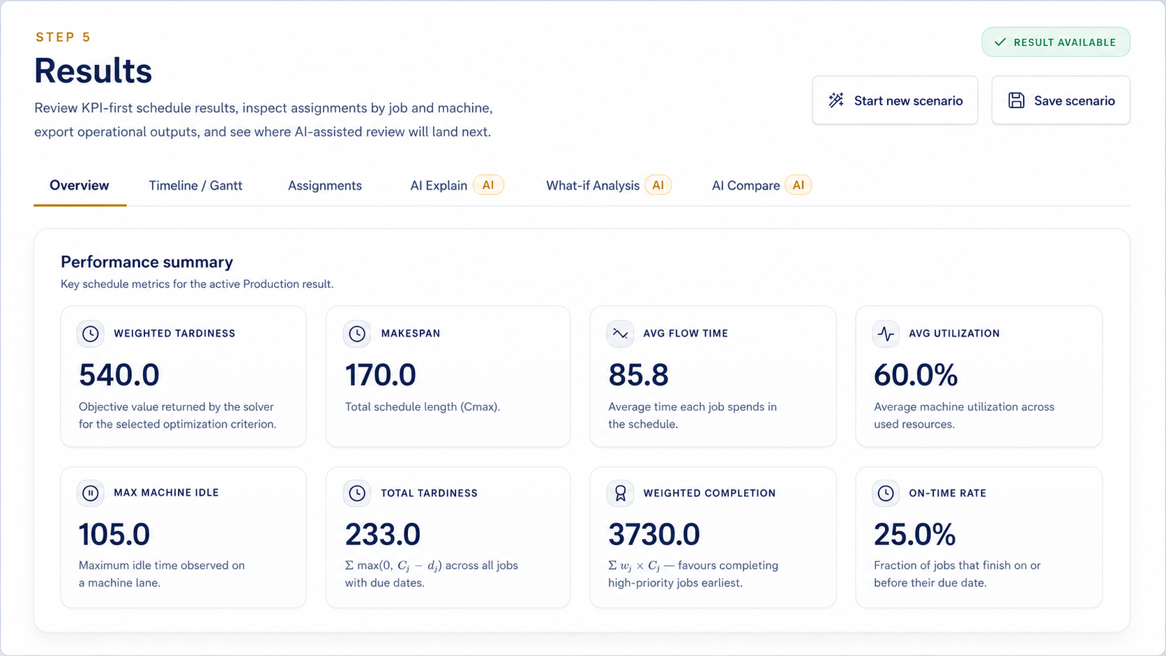
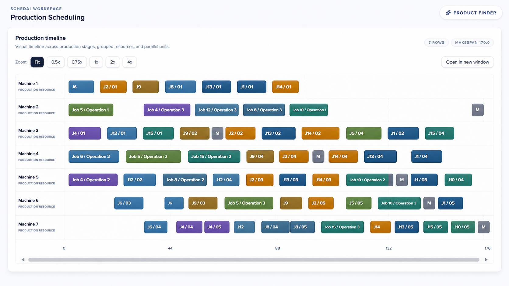
The result created a different schedule, but it did not improve the already-optimized 120-second scenario. Weighted tardiness increased from 495.0 to 540.0. Makespan increased from 168.0 to 170.0. Total tardiness increased from 222.0 to 233.0.
Average flow time increased from 81.2 to 85.8. Average utilization decreased from 61.1% to 60.0%, and maximum machine idle time increased from 100.0 to 105.0.
This showed that moving the maintenance window later did not automatically improve the schedule. Although the change appeared operationally reasonable, it introduced new trade-offs in the production plan.
| Metric | 120-sec solver | Maintenance shift |
|---|---|---|
| Weighted tardiness | 495.0 | 540.0 |
| Makespan | 168.0 | 170.0 |
| Total tardiness | 222.0 | 233.0 |
| Average flow time | 81.2 | 85.8 |
| Average utilization | 61.1% | 60.0% |
| Max machine idle | 100.0 | 105.0 |
AI Compare
AI Compare made the better scenario clear.
After running both what-if scenarios, the team used AI Compare to evaluate the results side by side.
The comparison focused on the 120-second solver scenario and the maintenance-window scenario. This allowed the team to answer a practical planning question: should they keep the improved optimizer result, or adopt the additional maintenance-window change?
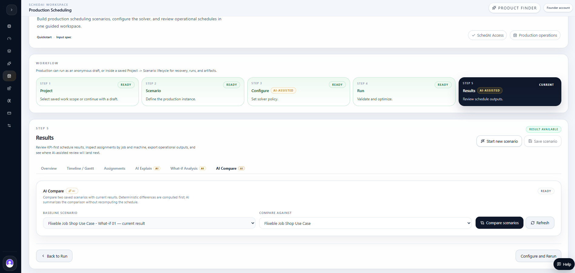
AI Compare showed that the 120-second solver scenario remained the stronger schedule.
Compared with the maintenance-shift scenario, the solver-time scenario reduced weighted tardiness from 540.0 to 495.0, shortened makespan from 170.0 to 168.0, improved average utilization from 60.0% to 61.1%, and reduced maximum machine idle time from 105.0 to 100.0.
Both scenarios scheduled the same 60 operations. This meant the difference was not caused by adding or removing work. The difference came from how operations were sequenced, assigned, and balanced across the machines.
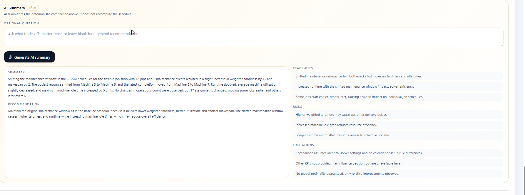
AI Compare also showed that the maintenance shift changed the structure of the schedule. Eight jobs moved earlier, four jobs moved later, and 17 operation assignments changed. The busiest resource shifted from Machine 3 to Machine 5, while the latest completion resource shifted from Machine 6 to Machine 7.
This helped the team understand that the maintenance shift did not simply free capacity. It changed the balance of the schedule and created a different production plan, but not a better one.
Case-study comparison summary
Scenario 1 stayed stronger after the maintenance-shift test.
Same environment, same objective, same operation count. The difference came from sequencing and resource balance.
Environment
Flexible Job Shop
Objective
Weighted Tardiness
Solver
CP-SAT
Runtime
120 seconds
Jobs
12
Operations
60
Machines
7
Maintenance tasks
6
| Metric | Scenario 1 | Scenario 2 | Result |
|---|---|---|---|
| Weighted tardiness | 495 | 540 | Scenario 1 |
| Makespan | 168 | 170 | Scenario 1 |
| Runtime | 59.95 s | 120.0 s | Scenario 1 |
| Average utilization | 61.05% | 60.0% | Scenario 1 |
| Max idle | 100 | 105 | Scenario 1 |
| Operations scheduled | 60 | 60 | Same scope |
KPI result
- Lower weighted tardiness.
- Shorter makespan.
- Lower maximum machine idle time.
- Slightly higher utilization.
Schedule changed
- 4 jobs moved earlier.
- 8 jobs moved later.
- 17 operation assignments changed.
Resource shifts
- Busiest resource moved from Machine 3 to Machine 5.
- Latest completion resource moved from Machine 6 to Machine 7.
- The change created a different plan, not a better one.
The operational decision was to keep Scenario 1 and reject the maintenance shift for this plan. The maintenance test remained useful because it showed how a realistic change would affect the schedule, but the measured KPIs did not support adopting it.
After the deterministic comparison was visible, the team could also use the AI Summary inside AI Compare to turn the KPI deltas and structural changes into a plain-language recommendation.
That summary did not replace the measured comparison. It helped the team explain why the stronger schedule should be kept and why the maintenance-shift variant should be treated as useful evidence, but not adopted.
Operational Decision
The team selected the 120-second solver scenario.
After reviewing the AI Compare results, the team selected the 120-second solver scenario as the preferred schedule.
The maintenance-window scenario was still useful because it showed how a realistic operational adjustment could affect the full production plan. However, the comparison showed that this change did not improve the selected KPIs. It created a different schedule, but not a better schedule.
Based on this result, the team decided not to move the maintenance window for this plan. Instead, they kept the stronger 120-second solver scenario and treated the maintenance shift as a rejected what-if scenario.
This helped the team make the scheduling decision based on measured performance rather than assumption. SchedAI did not only help the team identify a better schedule; it also helped them avoid a change that could have made the plan worse.
Final takeaway
This case study shows how SchedAI helps production teams move from static scheduling to decision-ready planning.
In a flexible job shop environment, the challenge is not only to create a feasible schedule. The real challenge is to understand whether that schedule is good enough, what trade-offs it creates, and which planning changes should be adopted before work reaches the production floor.
The key insight was that better scheduling is not always about making one obvious change. A schedule can improve makespan, tardiness, utilization, and idle time, while another realistic operational change may shift bottlenecks, move jobs later, or weaken the selected KPIs.
This is where SchedAI becomes valuable for production teams. It does not simply generate a schedule and leave the team to interpret it manually. It helps planners test scenarios, compare outcomes, understand trade-offs, and make a clearer decision before execution.
For teams managing complex production environments, SchedAI provides a practical way to ask: What if we change this? And more importantly: Is this change actually better?
Model a realistic flexible job shop with setup times, release times, due dates, priorities, and maintenance windows.
Generate a feasible production schedule that respects operation sequences, machine eligibility, and machine availability.
Use AI Explain to understand why the baseline schedule still had high tardiness and delivery pressure.
Test a stronger optimization scenario by increasing solver runtime from 60 seconds to 120 seconds.
Use AI Compare to determine whether a scenario truly improved the schedule or only changed the schedule structure.
Select the stronger scenario based on measurable KPIs rather than assumption.