

Executive Summary
Forecasting turned model comparison into a planning-ready weekly demand signal.
A distribution-center planning team needed a reliable weekly demand forecast before setting inventory, staffing, and capacity plans for the next quarter. The case used 208 weekly demand observations and tested both classical univariate forecasting and driver-aware machine learning.
The team trained SARIMA and ETS on the weekly demand history, then uploaded a multivariate dataset to test whether LightGBM could improve the forecast with promotion, price, traffic, holiday, backlog, capacity, and weather signals.
AI Compare kept the model-selection decision grounded. ETS and SARIMA were close on the weekly history, while the driver-aware LightGBM version produced weaker holdout performance for this planning run.
The team staged ETS as the practical project model, generated a 12-week W-MON forecast, and used AI Summary and AI Explain to turn the result into an inventory and staffing planning signal rather than a black-box prediction.
History
208 weekly rows
Models tested
SARIMA, ETS, LightGBM
Forecast
12 weekly steps
Core capabilities exercised
- Project-backed Forecast workspace with saved datasets, saved model versions, and run history.
- Univariate and multivariate time-series upload paths for classical and driver-aware models.
- SARIMA, ETS, and LightGBM training with persisted evaluation metrics and diagnostics.
- AI Compare for model-version review, including dataset lineage and comparability cautions.
- Staged-model execution so the preferred project model can be used consistently for forecasting.
- Forecast chart, table, provenance, and interval review for planning decisions.
- AI Summary and AI Explain to translate forecast evidence into operational implications.
Operating context
Forecasting had to support a model decision, not just draw a line.
Forecasting decisions are rarely only technical. Operations teams need to know what model was trained, what data it used, how it performed on recent holdout periods, and whether the resulting forecast is stable enough to support a planning decision.
In this case, the business question was weekly distribution-center demand. The team needed to anticipate near-term volume so inventory, staffing, carrier capacity, and warehouse planning could be reviewed before demand moved.
The workflow intentionally tested more than one modeling assumption. SARIMA and ETS represented classical univariate seasonal models. LightGBM represented a driver-aware machine learning path that could use numeric inputs such as promotion, price, traffic, holidays, backlog, capacity, and weather.
That made the use case stronger than a single-model demo. The team did not assume that more features would automatically produce a better forecast. They trained, compared, staged, and forecasted with evidence.
Forecasting challenge
The team needed evidence before choosing a model for planning.
The team did not just need a forecast line. They needed a defensible modeling workflow.
A simple seasonal model can be easier to explain and sometimes more stable. A driver-aware model can capture external signals, but only when the data and future assumptions are strong enough to justify that complexity.
The Forecasting workspace therefore had to support the full planning loop: upload data, train multiple saved versions, compare metrics and lineage, stage a practical model, generate a forward forecast, and explain the result in business language.
The workflow needed to prove
- Avoid treating the first trained model as the default answer.
- Compare SARIMA, ETS, and LightGBM using persisted holdout evidence.
- Keep dataset lineage visible when models use different data versions.
- Distinguish staged model from automatically best model.
- Generate weekly timestamps that match the W-MON training frequency.
- Explain forecast uncertainty without turning it into a guarantee.
Method: Data setup
The team tested both univariate history and driver-aware data.
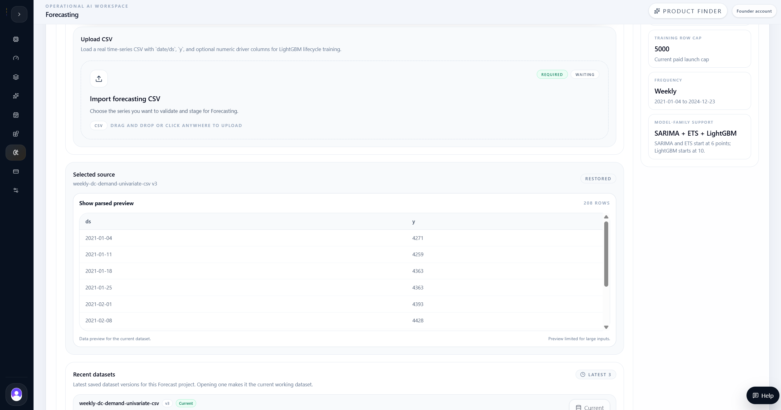
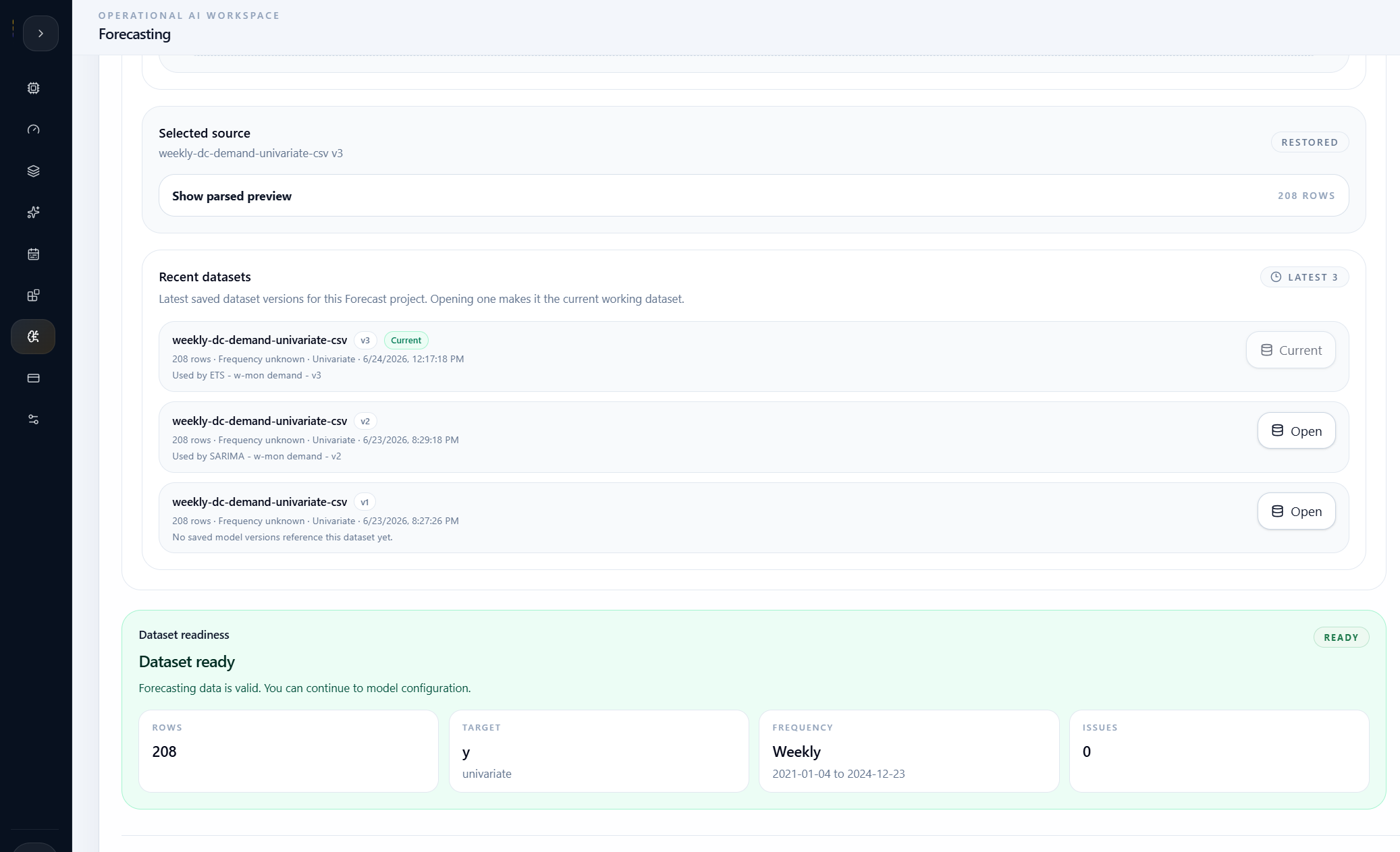
The planning team first loaded the univariate weekly demand history. That dataset supported SARIMA and ETS training with a clean date and target structure.
The team then loaded a multivariate version of the same demand problem to test LightGBM. The multivariate data included the target demand plus operational driver columns for promotions, pricing, site traffic, holiday flags, backlog, carrier capacity, and weather.
This made the model comparison useful. The team could test whether adding drivers improved the forecast, while the product preserved lineage so the model history remained transparent.
Dataset scope
- 208 weekly demand rows.
- Univariate file for SARIMA and ETS.
- Multivariate file for LightGBM.
- Target column: weekly distribution-center demand.
- Driver columns: promotion, price, site traffic, holiday, backlog, carrier capacity, and weather.
- Dataset lineage retained for model comparison.
Method: Train models
SARIMA, ETS, and LightGBM were trained as saved model versions.
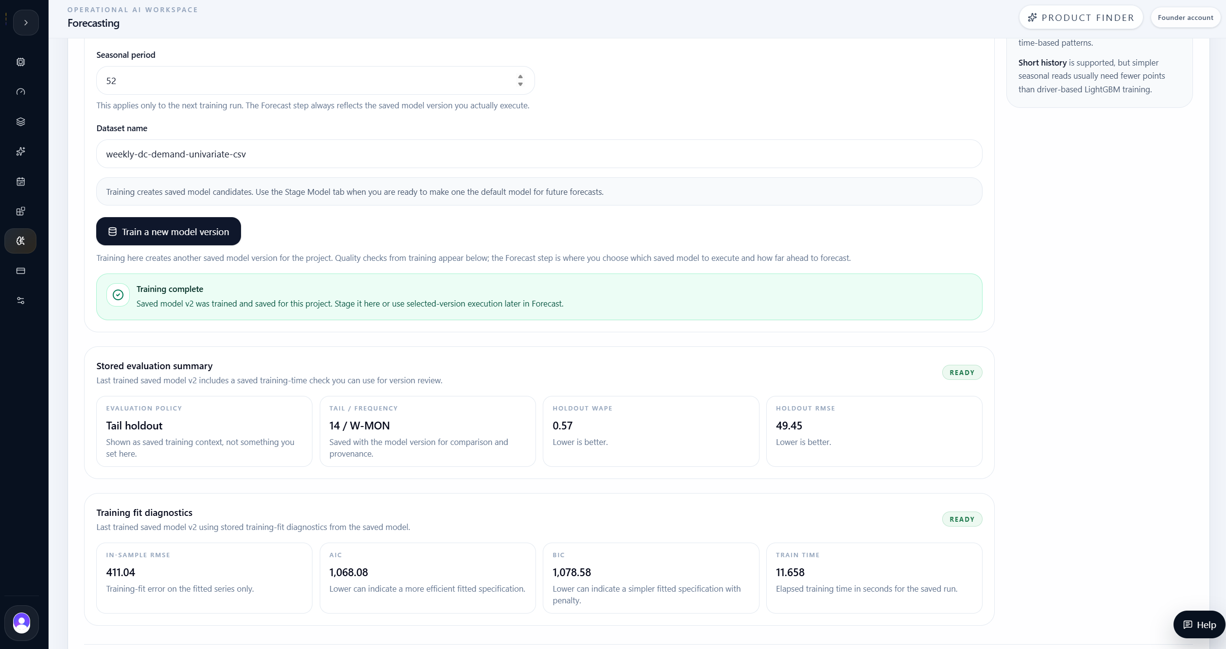
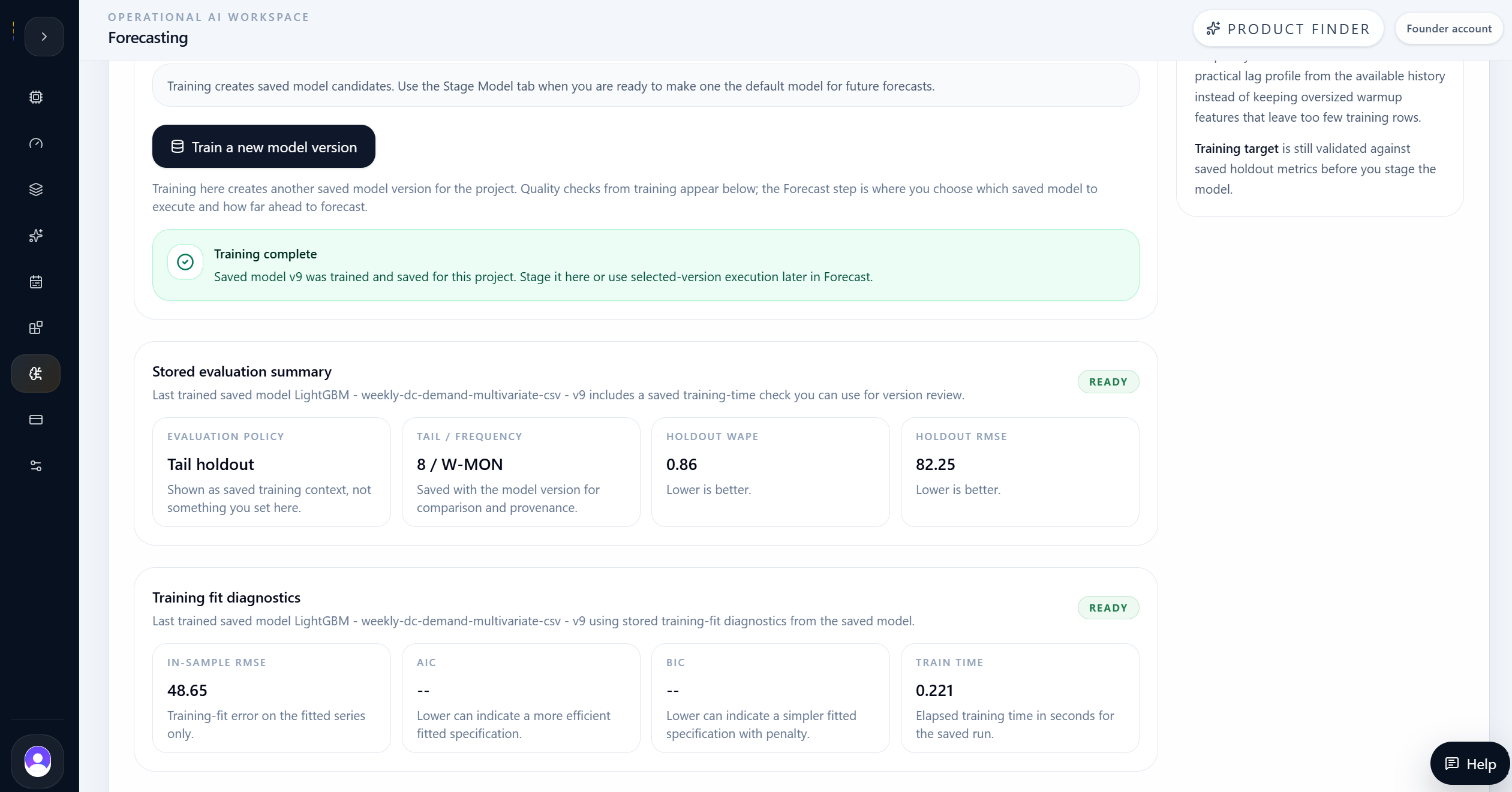
The team trained three saved versions. SARIMA and ETS used the univariate weekly history, while LightGBM used the multivariate history with driver columns.
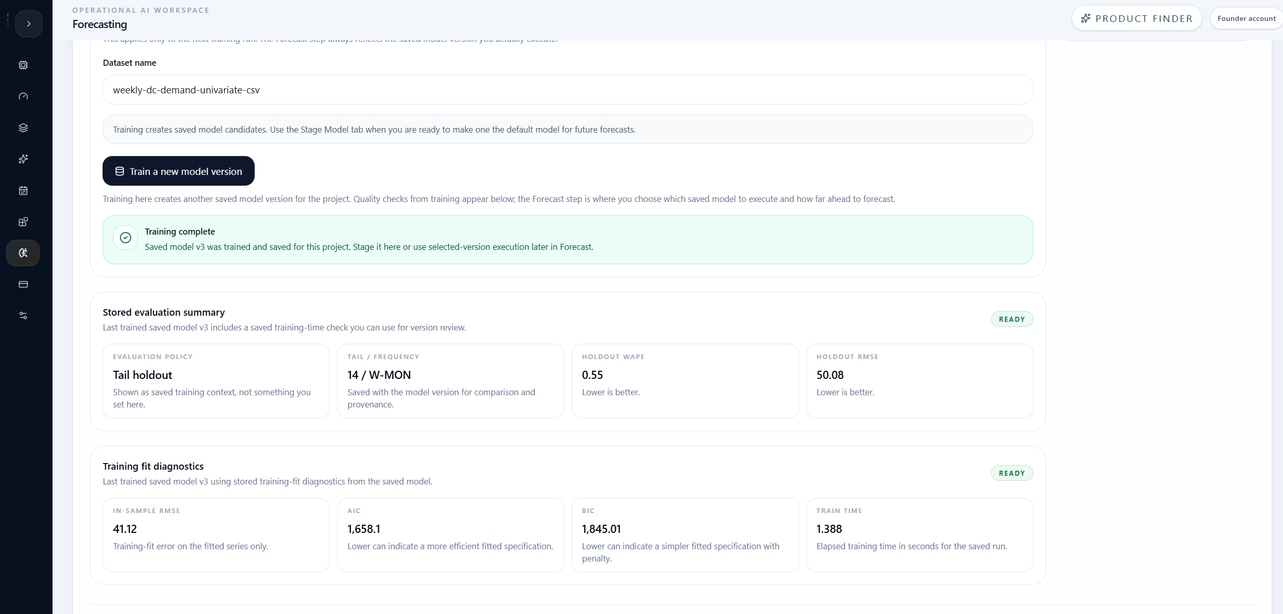
Training did more than create artifacts. Each saved version carried evaluation summaries and diagnostics so the team could compare quality before staging a model for forecasting.
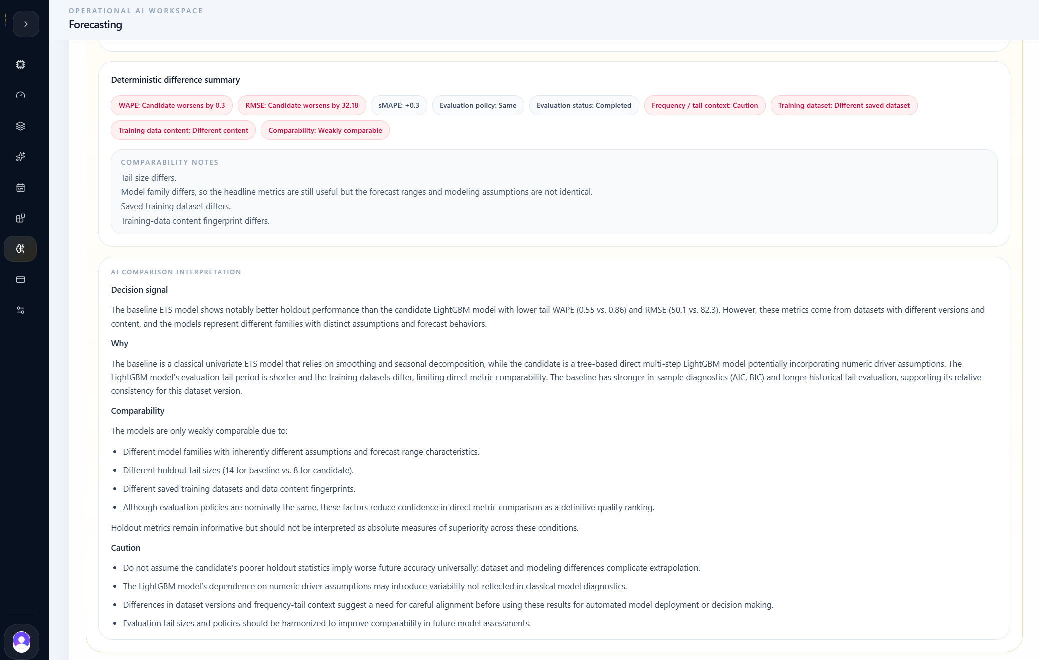
LightGBM was not dismissed because it was more complex. It was tested directly. The result showed that the driver-aware model was feasible, but its holdout WAPE and RMSE were weaker than the staged ETS result for this use case.
Training evidence captured
- SARIMA captured seasonal univariate structure.
- ETS captured level, trend, and weekly seasonal smoothing.
- LightGBM tested numeric driver-aware forecasting.
- Saved versions retained model family, dataset lineage, frequency, holdout policy, and metrics.
- Model names made versions easier to interpret during comparison.
Model comparison
AI Compare showed why richer inputs did not automatically win.
Terms used in this comparison
Holdout
Recent historical periods held back from training so the model can be tested on data it did not fit directly.
WAPE
Weighted Absolute Percentage Error. Lower values mean the forecast missed less demand volume relative to the actual volume.
RMSE
Root Mean Squared Error. Lower values mean fewer large forecast misses in the holdout window.
SARIMA
A seasonal statistical forecasting model that uses the demand history itself.
ETS
A statistical smoothing model for level, trend, and seasonality. It is often practical when the seasonal pattern is stable.
LightGBM
A tree-based machine learning model that can use extra driver columns such as promotion, price, traffic, holidays, backlog, and capacity.
W-MON
Weekly forecast frequency where each forecast timestamp lands on a Monday.
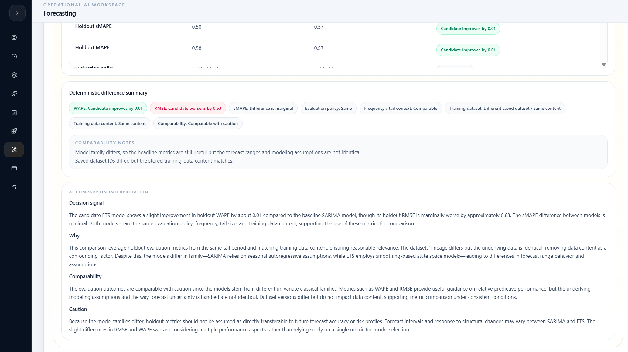
The first AI Compare pass evaluated SARIMA against ETS on the weekly demand history. The models were close, but ETS became the practical candidate to stage because it provided a strong, interpretable smoothing path with stable forecast ranges.
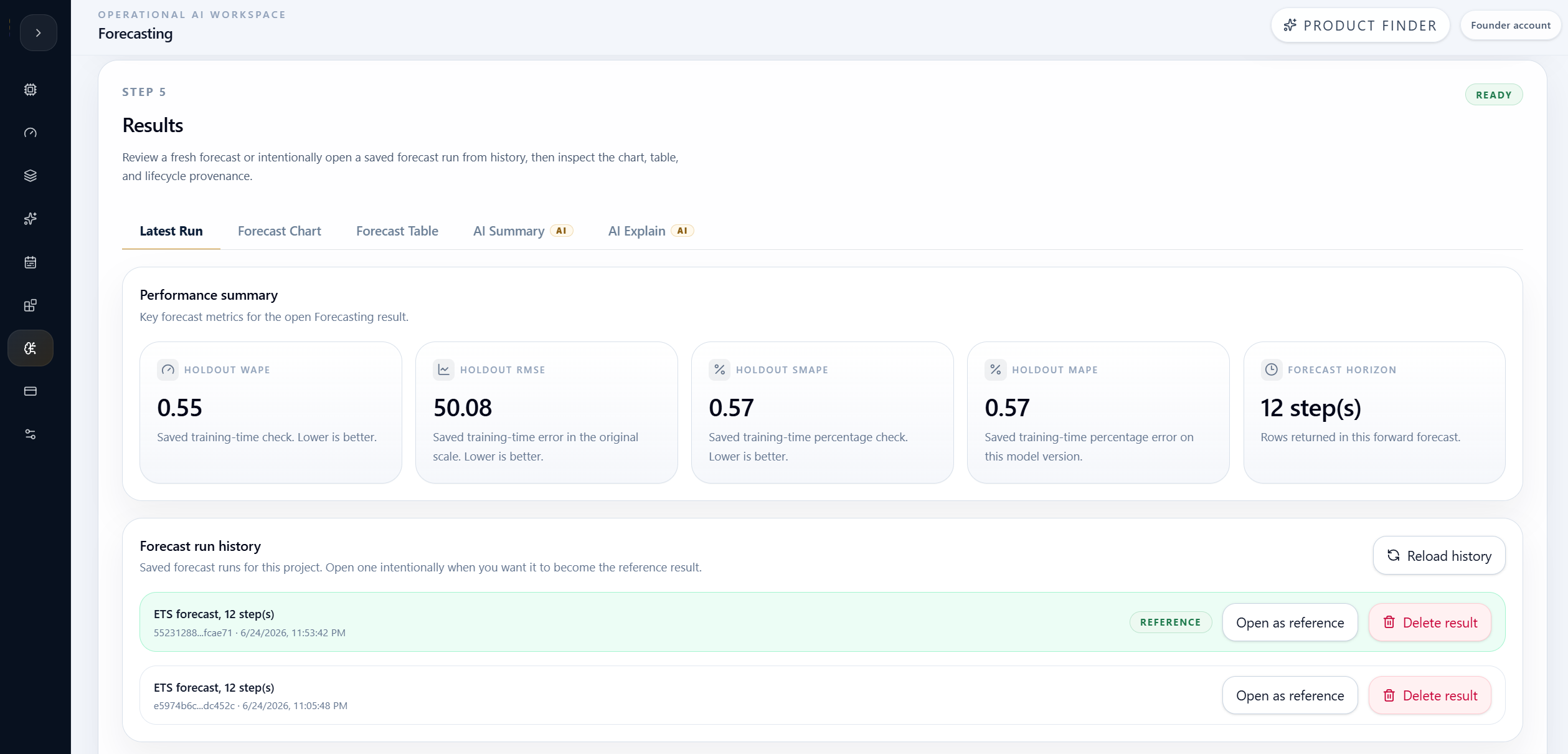
The second AI Compare pass tested LightGBM against ETS. LightGBM had the richer driver-aware dataset, but the comparison showed weaker holdout metrics: LightGBM WAPE around 0.86 and RMSE around 82.25, versus ETS WAPE around 0.55 and RMSE around 50.08.
That was the useful product signal. The driver-aware model was not rejected because it used different inputs. It was rejected for this forecast run because its measured holdout error was materially worse and the added model complexity did not buy better planning accuracy.
Model set
SARIMA, ETS, LightGBM
ETS staged
Lowest holdout error
Holdout WAPE
ETS 0.55
LightGBM 0.86
ETS missed less demand volume
Forecast horizon
12 future weeks
Weekly W-MON
Planning cadence preserved
| Evidence | Result |
|---|---|
| Best staged candidate | ETS |
| ETS holdout WAPE | 0.55 |
| ETS holdout RMSE | 50.08 |
| SARIMA position | Close second on the same weekly univariate history |
| LightGBM test | Driver-aware model with promotion, price, traffic, holiday, backlog, capacity, and weather inputs |
| LightGBM holdout WAPE | 0.86 |
| LightGBM holdout RMSE | 82.25 |
| Decision signal | Stage ETS because it had lower error and simpler operating assumptions for this run |
Staged model
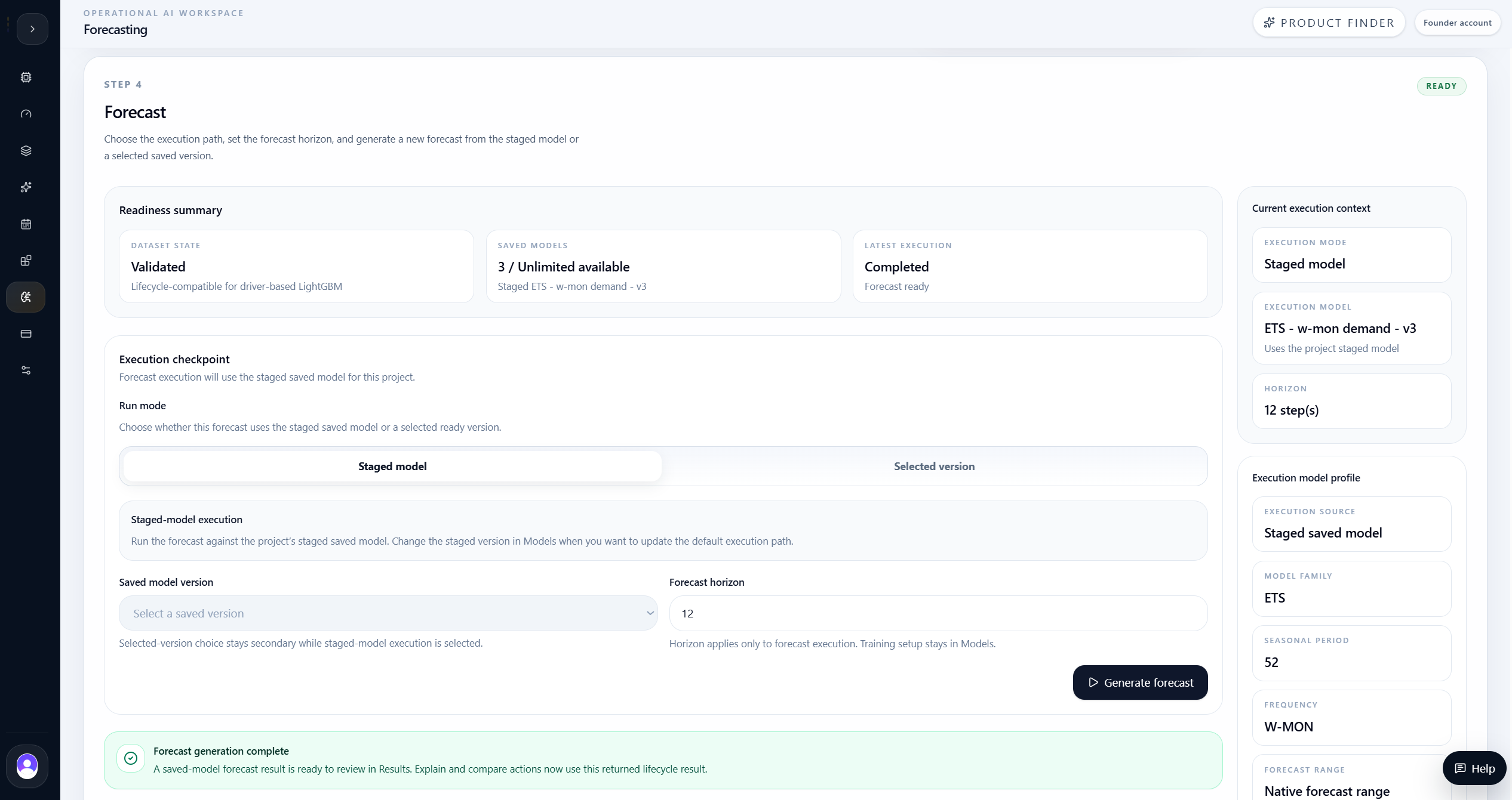
The team staged ETS as the project execution model.
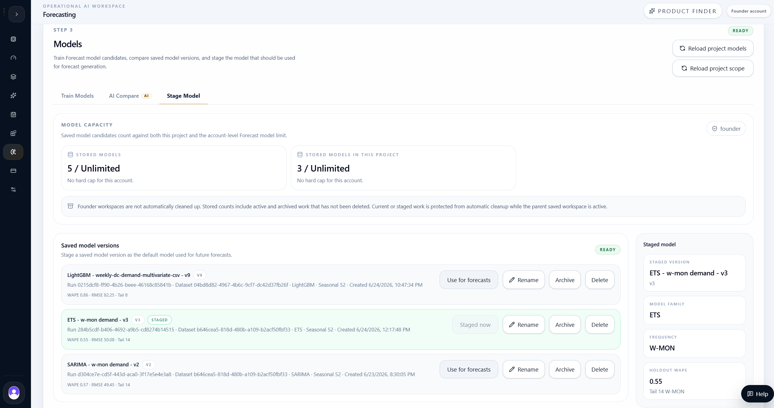
After reviewing the comparison evidence, the team staged ETS - w-mon demand - v3 as the project execution model.
That is an important product behavior. Staging does not mean the system magically declares a champion. It means the team selected the saved version they wanted to use as the project default for forecast execution.
For this case, the staged ETS model was a practical choice because it combined strong holdout performance, simple univariate interpretation, weekly frequency alignment, and stable forecast intervals.
Staging semantics
A staged model is the model the project will use by default for execution. It is selected by the team, not automatically crowned by the platform.
In this case, ETS was staged because the comparison evidence made it the practical choice for the 12-week forecast run.
Forecast result
The staged ETS model generated a 12-week W-MON forecast.
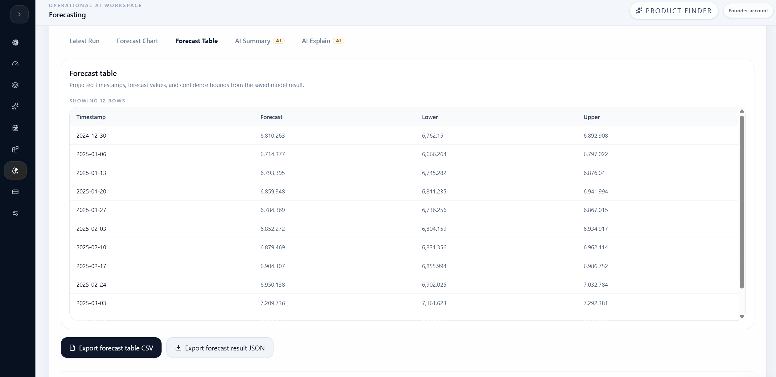
The team generated a 12-step forecast from the staged ETS model. The result preserved the weekly W-MON frequency, producing weekly timestamps from late December 2024 into March 2025.
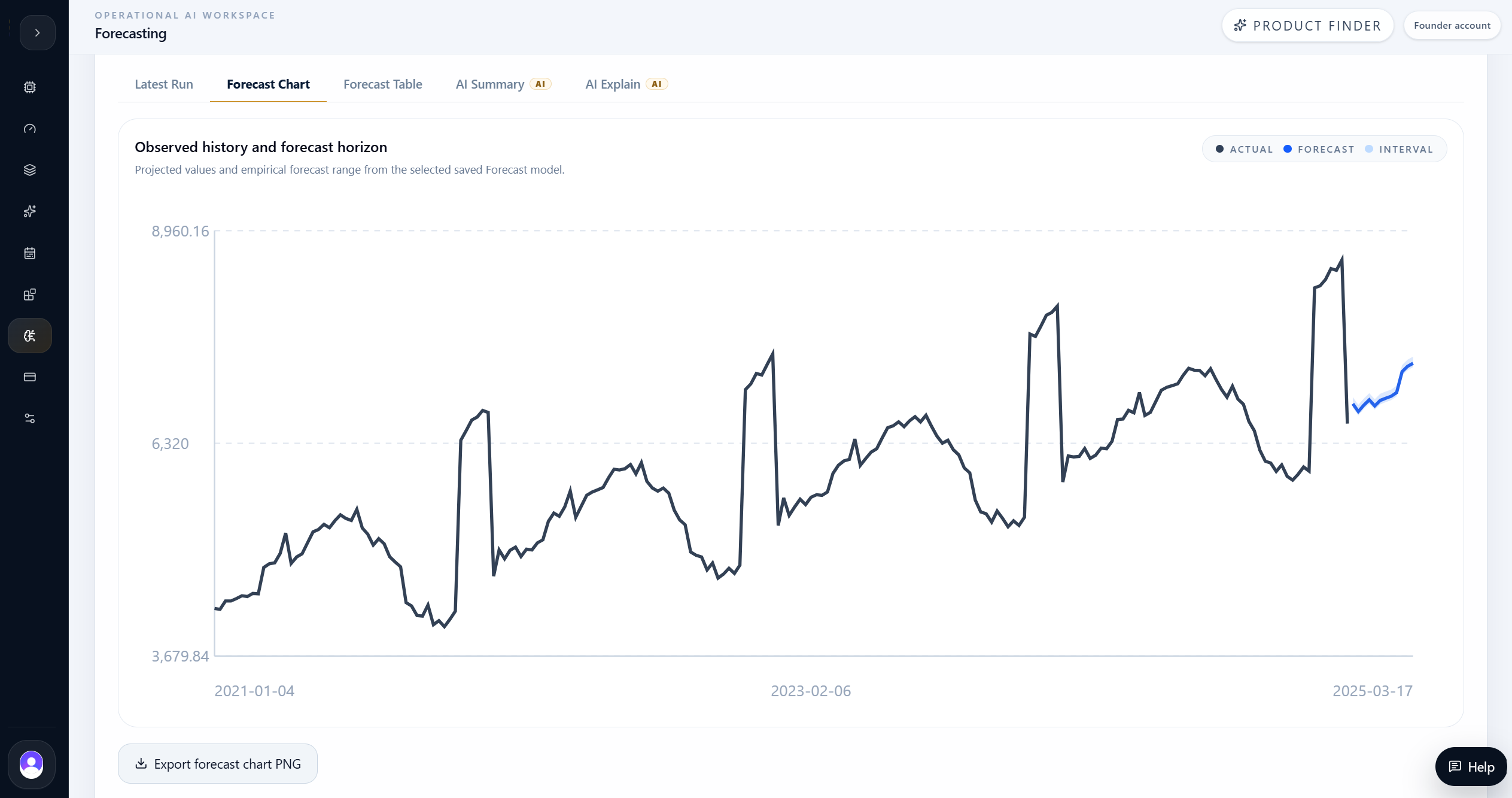
The forecast projected gradual demand growth from about 6,810 units at the start of the horizon to about 7,314 units by mid-March 2025.
The result included forecast values, lower and upper ranges, model provenance, holdout metrics, and a chart that made the observed history and forecast horizon easy to review.
| Forecast KPI | Value |
|---|---|
| Forecast horizon | 12 weekly steps |
| Frequency | W-MON |
| Model family | ETS |
| Seasonal period | 52 |
| Holdout WAPE | 0.55 |
| Holdout RMSE | 50.08 |
| Interval width | about +/-65 units |
AI Summary
AI Summary turned forecast output into operating context.
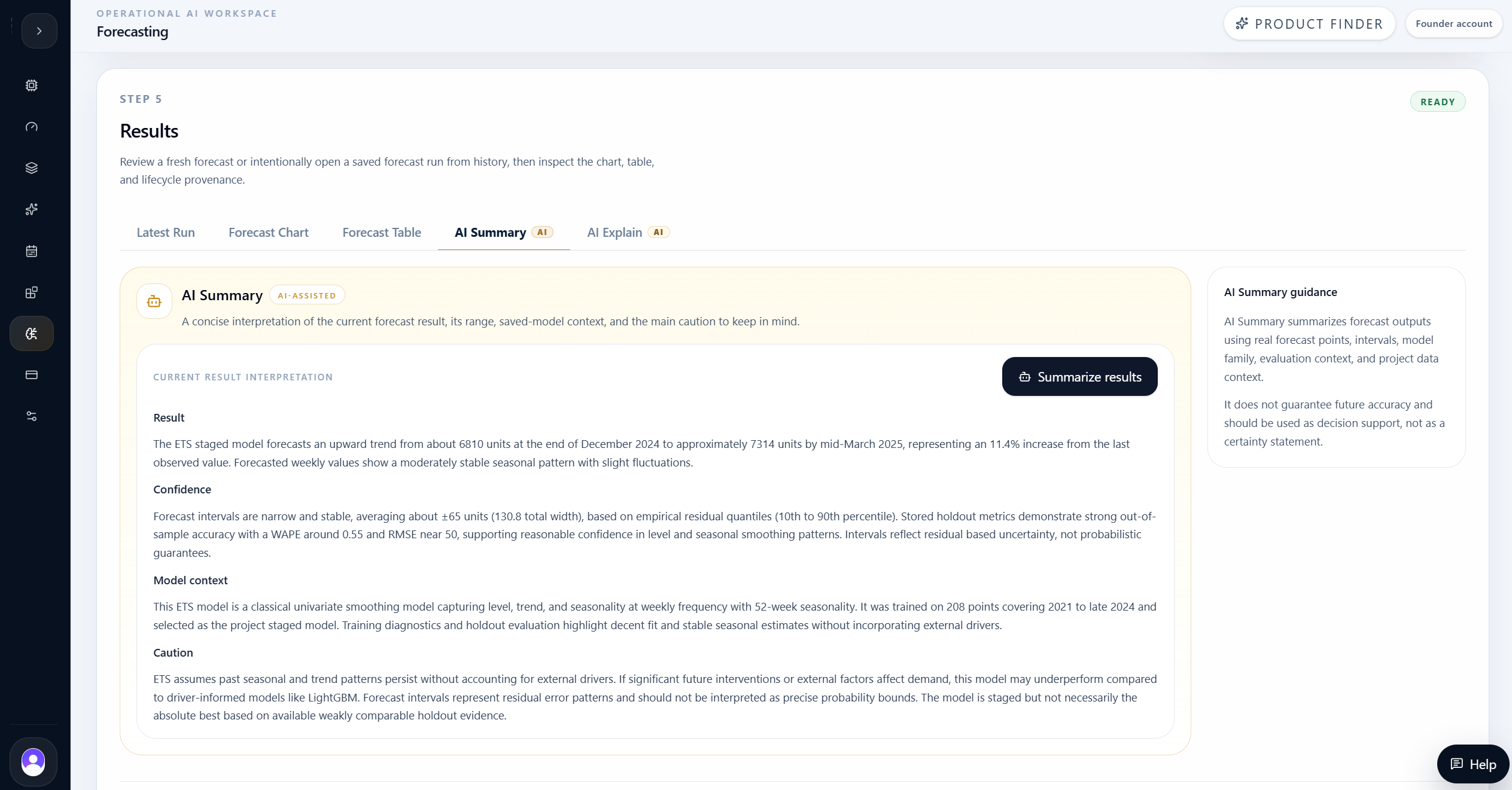
AI Summary translated the forecast into a concise operating interpretation. It described the upward weekly demand trend, the moderate and stable uncertainty range, and the role of the staged ETS model.
The summary also included the right caution. ETS assumes historical level, trend, and seasonality remain informative. If future promotions, capacity disruptions, or other external factors materially shift demand, a driver-aware model may deserve another review.
That is the right kind of forecasting assistant behavior. It supports a decision without pretending the forecast is a guaranteed future outcome.
AI Explain
AI Explain connected the forecast to inventory and staffing decisions.
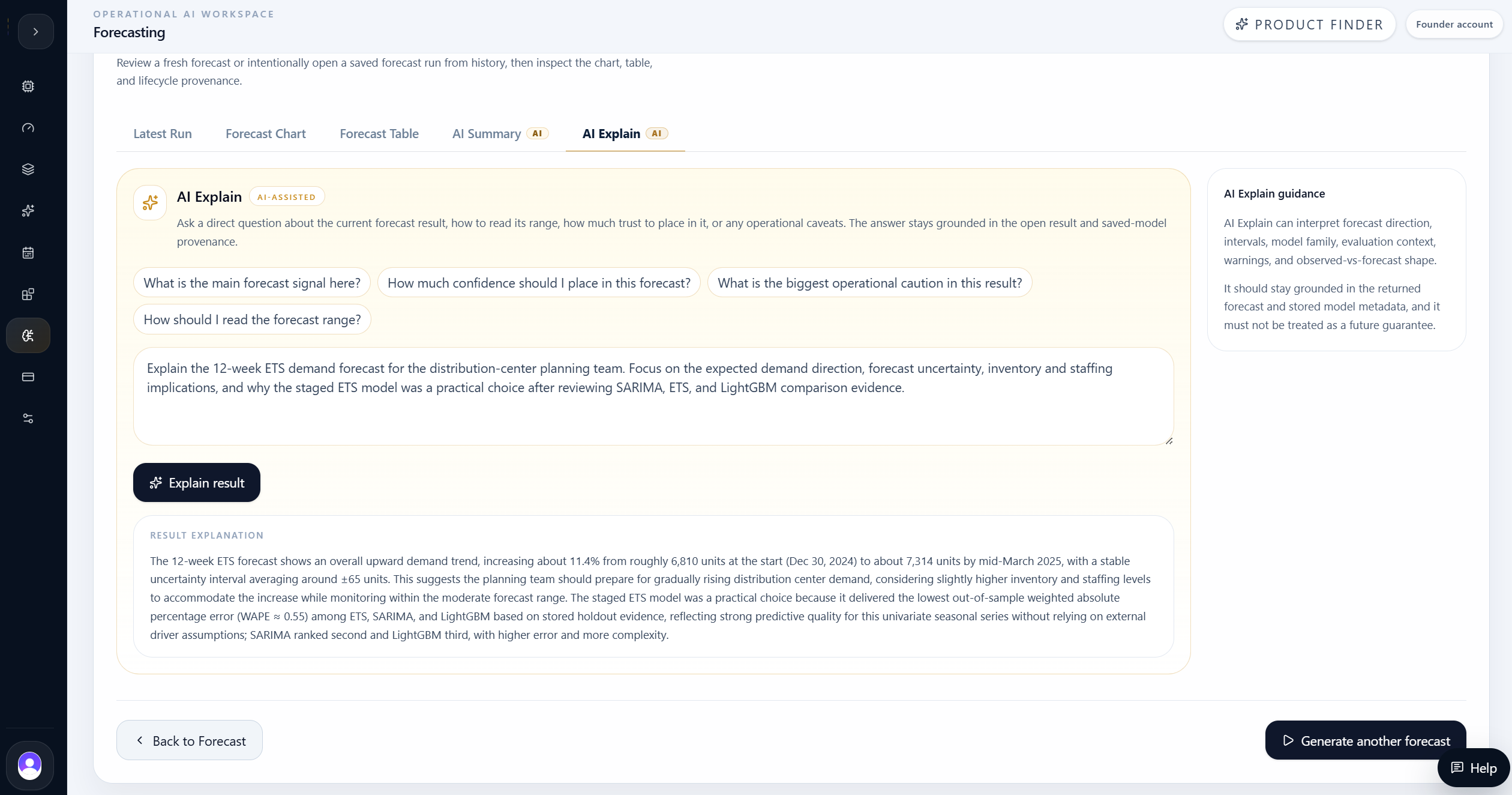
AI Explain answered a planning-specific question: what does this 12-week ETS forecast mean for the distribution-center team, and why was the staged ETS model a practical choice after reviewing SARIMA, ETS, and LightGBM evidence?
The answer connected the forecast signal to inventory and staffing. Demand was expected to rise gradually, so the team should prepare for higher warehouse volume while monitoring the forecast range.
It also explained the model decision: ETS had the strongest stored holdout evidence for this use case, SARIMA was close, and LightGBM was less attractive because its higher error and added complexity did not justify staging it for this forecast run.
Planning decision
The team used ETS to support near-term distribution-center planning.
The team used ETS as the planning model for this weekly distribution-center forecast.
The decision was not based on model fashion. It was based on a complete product workflow: train classical and driver-aware candidates, compare saved versions, preserve lineage, stage the practical model, run a weekly forecast, and ask AI to explain the result in planning language.
The final planning signal was clear enough to act on carefully: demand is trending upward across the next 12 weekly periods, intervals remain relatively narrow, and the team should prepare inventory and staffing capacity while watching for external changes that could invalidate the historical seasonal pattern.
For operations teams, this is the value of Forecasting inside MAG OptiAI: it turns raw time-series data into a reviewable model-selection and forecasting workflow, not just a chart.
Final takeaway
The best story was not that LightGBM was bad or ETS is always better. The product showed that the right model depends on evidence, lineage, and the planning question.
For this weekly demand case, ETS was the practical model to stage and run. The result gave the team a grounded capacity signal for the next 12 weeks.
Model comparison matters more than model complexity.
Dataset lineage prevents misleading apples-to-oranges conclusions.
Staged model means selected execution model, not automatically best model.
Weekly frequency and forecast timestamps stayed aligned.
AI Summary and AI Explain made the forecast usable for inventory and staffing planning.